Low-level access to IRIS data in Python
Contents
8. Low-level access to IRIS data in Python#
In some cases it is better to focus on simple and efficient methods that do not make use of higher-level abstractions or IRIS-specific packages such as that have been described here. The motivation could be two-fold: To detail a “bare bones” interface when no other packages are available, or when performance is the goal, and secondly to provide a simple guide while irispy-lmsal is not mature enough to provide a stable API.
One can use the earlier chapters in this guide as a starting point for downloading (Searching and acquiring IRIS Level 2 data) and reading IRIS data (Working with IRIS Level 2 data in Python) into a Python session, but once that is done (or if one wants to read the IRIS raster and SJI FITS files directly using astropy) one can work with the data directly.
A practical guide has been written explaining how to read and analyze data from IRIS, using Python at this simple level is available Low level guide to IRIS using Python. The guide has the very nice fact that the tutorial itself is written as a Jupyter notebook, so it can be run in that environment, or if one prefers in e.g., an IPython session.
We will repeat a slightly shortened version of the tutorial here, where we instead of using astropy FITS reader directly, we use the methods described in the first chapters of this guide. The two worked examples are missing as well, and we strongly recommend that the reader will look at the those.
8.1. Requirements#
To follow the Low level guide to IRIS using Python guide only standard python scientific packages are necessary:
8.2. Reading IRIS files#
The IRIS level 2 FITS files are the standard science data product, and can be read with any standard FITS reader. Here we make use of the routines discussed previous chapters manual instead of using astropy.io.fits directly.
For this part we will make use of a dataset from 2018-01-02. Please download the data files and unpack them in your working directory. The commands used here will assume you are at the directory with the IRIS FITS files.
We’ll start by setting up matplotlib and importing the level 2 reader.
Here we use the inline backend, but for interactive use you should use ipympl.
>>> # %matplotlib inline
>>> import numpy as np
>>> import iris_lmsalpy.hcr2fits as hcr2fits
>>> import iris_lmsalpy.extract_irisL2data as ei
>>> from matplotlib import colors, cm, pyplot as plt
>>> from astropy.wcs import WCS
>>> from astropy import units as u

>>> # Set up some default matplotlib options
>>> plt.rcParams['figure.figsize'] = [10, 6]
>>> plt.rcParams['xtick.direction'] = 'out'
>>> plt.rcParams['image.origin'] = 'lower'
>>> plt.rcParams['image.cmap'] = 'viridis'
8.2.1. Reading level 2 SJI files#
Let us open a SJI file from the 1400 filter.
>>> SJI_filename = 'iris_l2_20180102_153155_3610108077_SJI_1400_t000.fits'
>>> sji = ei.load(SJI_filename)
The provided file is a SJI IRIS Level 2 data file containing SJI_1400 data.

Extracting information from file iris_l2_20180102_153155_3610108077_SJI_1400_t000.fits...

Available data with size Y x X x Image are stored in a windows labeled as:

-------------------------------------------------------------
Index --- Window label --- Y x X x Im --- Spectral range [AA]
-------------------------------------------------------------
    0         SJI_1400       548x845x80     1380.00 - 1420.00
-------------------------------------------------------------

Observation description:  Very large dense 320-step raster 105.3x175 320s   Deep x 8 Spatial x
The SJI data are passed to the output variable, e.g., iris_data, as a dictionary with the following entries:
iris_data.SJI['SJI_1400']
The data itself and some metadata is contained in the SJI object as shown earlier, but we can extract the main header (or auxiliary headers using the extent keyword; see ITN 26 on structure of level 2
files).
We can have a look at the main header, which is in the first HDU:
>>> hd = ei.only_header(SJI_filename, verbose = True)
Reading file iris_l2_20180102_153155_3610108077_SJI_1400_t000.fits...
Filename: iris_l2_20180102_153155_3610108077_SJI_1400_t000.fits
No.    Name      Ver    Type      Cards   Dimensions   Format
0  PRIMARY       1 PrimaryHDU     162   (845, 548, 80)   int16 (rescales to float32)
1                1 ImageHDU        38   (31, 80)   float64
2                1 TableHDU        33   80R x 5C   [A10, A10, A3, A66, A55]

Observation description:  Very large dense 320-step raster 105.3x175 320s   Deep x 8 Spatial x

Extension No. 1 stores data and header of SJI_1400: 1380.00 - 1420.00 AA

To get the main header use :
hdr = extract_iris2level.only_header(filename)

To get header corresponding to data of SJI_1400 use :
hdr = ei.only_header(filename, extension = 0)

To get the data of SJI_1400 use :
data = ei.only_data(filename, extension = 0, memmap = True)

Returning header for extension No. 0

>>> hd
SIMPLE  =                    T / Written by IDL:  Tue Mar 20 23:39:27 2018
BITPIX  =                   16 / Number of bits per data pixel
NAXIS   =                    3 / Number of data axes
NAXIS1  =                  845 /
NAXIS2  =                  548 /
NAXIS3  =                   80 /
EXTEND  =                    T / FITS data may contain extensions
DATE    = '2018-03-21'         / Creation UTC (CCCC-MM-DD) date of FITS header
COMMENT FITS (Flexible Image Transport System) format is defined in 'Astronomy
COMMENT and Astrophysics', volume 376, page 359; bibcode 2001A&A...376..359H
TELESCOP= 'IRIS    '           /
INSTRUME= 'SJI     '           /
DATA_LEV=              2.00000 /
LVL_NUM =              2.00000 /
VER_RF2 = 'L12-2017-08-04'     /
DATE_RF2= '2018-03-21T06:00:07.640' /
DATA_SRC=              1.51000 /
ORIGIN  = 'SDO     '           /
BLD_VERS= 'V9R1X   '           /
LUTID   =              0.00000 /
OBSID   = '3610108077'         /
OBS_DESC= 'Very large dense 320-step raster 105.3x175 320s   Deep x 8 Spatial x'
OBSLABEL= '        '           /
OBSTITLE= '        '           /
DATE_OBS= '2018-01-02T15:32:23.340' /
...
CTYPE1  = 'HPLN-TAN'           /
CTYPE2  = 'HPLT-TAN'           /
CTYPE3  = 'Time    '           /
CUNIT1  = 'arcsec  '           /
CUNIT2  = 'arcsec  '           /
CUNIT3  = 'seconds '           /
KEYWDDOC= 'http://www.lmsal.com/iris_science/irisfitskeywords.pdf' /
HISTORY iris_prep  Set 1 saturated pixels to Inf
HISTORY iris_prep  Dark v20130925; T=[-59.1,-59.0,-58.3,-59.3,1.4,2.7,2.7,2.7,2.
HISTORY iris_prep  Flat fielded with recnum     440
HISTORY iris_prep  Set permanently bad pixels to 0 prior to warping
HISTORY iris_prep_geowave_roi  ran with rec_num 4
HISTORY iris_prep_geowave_roi  boxwarp set to 1
HISTORY iris_prep_geowave_roi  updated WCS parameters with iris_isp2wcs
HISTORY iris_prep  Used iris_mk_pointdb ver 10
HISTORY iris_prep       Fiducial midpoint shift X,Y [pix]:      0.22    -0.17
HISTORY iris_prep  Used INF_POLY_2D for warping
HISTORY iris_prep VERSION:  1.96
HISTORY iris_prep   ran on 20180321_063639
HISTORY level2  Version L12-2017-08-04
Header entries can be accessed like a dictionary. For example, for the start of the slit-jaw sequence:
>>> hd['STARTOBS']
'2018-01-02T15:31:55.700'
The data are stored under sji.SJI['SJI_1400'].data.
You can see that NAXIS1=845 (spatial x), NAXIS2=548 (spatial y), and NAXIS3=80 (time).
In Python the arrays are in C order, dimension order will be reversed:
>>> sji.SJI['SJI_1400'].data.shape
(80, 548, 845)
We can plot the first timestep to see what it looks like:
>>> plt.imshow(sji.SJI['SJI_1400'].data[...,0])
>>> plt.show()
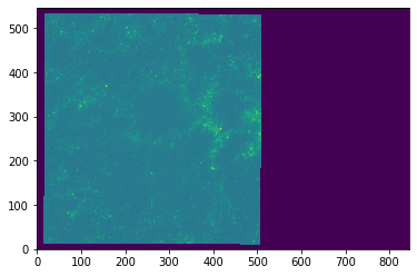
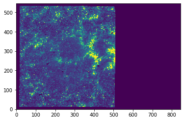
The image looks washed out because of the automatic scaling. We can get a better scaling by adjusting the maximum and minimum range:
>>> plt.imshow(sji.SJI['SJI_1400'].data[...,0],vmin=0, vmax=100)
>>> plt.show()
In some cases, loading the whole data into memory may not be practical. For this, it is possible to use an approach based on numpy.memmap that allows us to load only parts of the data, and only when necessary. Refer to the first chapters of this guide, or the original tutorial on low-level python processing for details.
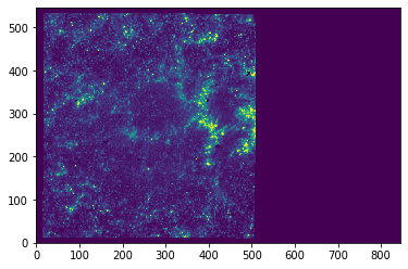
Let us show another method for scaling the data based on histogram optimization.
>>> import iris_lmsalpy.im_view as im

>>> lev=im.histo_opt(sji.SJI['SJI_1400'].data[...,0])
-2.00e+02/3.24e+02 image min/image max
5.71e+00/1.40e+02 histo_opt min/histo_opt max

>>> plt.imshow(sji.SJI['SJI_1400'].data[...,0],vmin=lev[0], vmax=lev[1])
>>> plt.show()
8.2.1.1. Coordinates#
So far, we have used plt.imshow directly, which shows the data in pixel values.
Coordinate information is available in the SJI header, with the World Coordinate System (WCS) keywords.
astropy package has a wcs module that allows plotting the image with the proper solar (X, Y) coordinates.
First we get the WCS data from the SJI header:
>>> from astropy.wcs import WCS
>>> wcs = WCS(hd)
WARNING: FITSFixedWarning: 'unitfix' made the change 'Changed units:
    'seconds' -> 's'. [astropy.wcs.wcs]
Inspecting this object we see:
>>> wcs
WCS Keywords

Number of WCS axes: 3
CTYPE : 'HPLN-TAN'  'HPLT-TAN'  'Time'
CRVAL : -0.09147805555555556  0.07962555555555555  1463.91
CRPIX : 423.0  274.5  40.0
PC1_1 PC1_2 PC1_3  : 0.99997061491  0.0112785818055  0.0
PC2_1 PC2_2 PC2_3  : -0.0112785818055  0.99997061491  0.0
PC3_1 PC3_2 PC3_3  : 0.0  0.0  1.0
CDELT : 9.241666666666666e-05  9.241666666666666e-05  36.8284
NAXIS : 845  548  80
We can see that the first two axes have type of ‘HPLN’ and ‘HPLT’, meaning HelioProjective-Cartesian longitude and latitude respectively, or solar X and Y. The last axis is time in seconds.
It should also be noted that the main SJI header is the average of the individual WCS for each slit-jaw image.
You will need to account for the correct XCEN and YCEN values from the auxiliary header and data array.
To plot the coordinate axes in matplotlib, we do the following:
>>> ax = plt.subplot(projection=wcs.dropaxis(-1))
>>> ax.imshow(sji.SJI['SJI_1400'].data[...,0], vmin=lev[0], vmax=lev[1])
>>> plt.show()
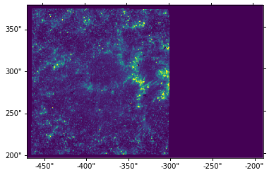
We do wcs.dropaxis(-1) because we do not want to plot the time coordinate.
We can also overplot the coordinates grid by calling ax.grid.
For the final figure with grid, we do:
>>> ax = plt.subplot(projection=wcs.dropaxis(-1))
>>> ax.grid(color='w', ls=':')
>>> ax.imshow(sji.SJI['SJI_1400'].data[...,0], vmin=lev[0], vmax=lev[1])
>>> plt.show()

You’ll notice that the solar coordinate grid is slightly tilted from the image axes. This is normal. With different IRIS roll angles, this difference will be even more obvious.
8.2.2. Reading level 2 raster files#
IRIS level 2 spectrograph files have a different structure from the SJI files. The main header is similar, but the data are all saved in extension HDUs. The reason for this is that spectrograph level 2 files are organised by spectral windows, which may differ for various observations.
Using the raster file from our example above, we can open the files with the methods described above and in previous chapters:
>>> raster_filename = 'iris_l2_20180102_153155_3610108077_raster_t000_r00000.fits'
>>> sp = ei.load(raster_filename)
The provided file is a raster IRIS Level 2 data file.

Extracting information from file /Users/asainz/iris_l2_20180102_153155_3610108077_raster_t000_r00000.fits...
Extracting information from file iris_l2_20180102_153155_3610108077_raster_t000_r00000.fits...

Available data with size Y x X x Wavelength are stored in windows labeled as:

--------------------------------------------------------------------
Index --- Window label --- Y x X x WL --- Spectral range [AA] (band)
--------------------------------------------------------------------
    0      C II 1336         548x320x335     1331.77 - 1340.44  (FUV)
    1      O I 1356          548x320x414     1346.75 - 1357.47  (FUV)
    2      Si IV 1394        548x320x195     1391.20 - 1396.14  (FUV)
    3      Si IV 1403        548x320x338     1398.12 - 1406.70  (FUV)
    4      2832              548x320x60      2831.34 - 2834.34  (NUV)
    5      2814              548x320x76      2812.65 - 2816.47  (NUV)
    6      Mg II k 2796      548x320x380     2790.65 - 2809.95  (NUV)
--------------------------------------------------------------------

Observation description:  Very large dense 320-step raster 105.3x175 320s   Deep x 8 Spatial x
The selected data are passed to the output variable (e.g iris_data) as a dictionary with the following entries:
iris_data.raster['Mg II k 2796']
The same comment made about memmap applies as for the SJI files, and is more important in the raster files because they tend to be larger.
The first FITS HDU has the main header. We can use it to find out what kind of raster this is:
>>> hd = ei.getheader(raster_filename)
>>> hd['OBS_DESC']
'Very large dense 320-step raster 105.3x175 320s   Deep x 8 Spatial x'
The number of FITS units in sp is the number of spectral windows plus 3 (additional metadata).
In this case we have 10 FITS units, so 7 spectral windows.
We can also look at the “NWIN” keyword in the main header.
Let us work with the “Mg II k 2796” window, which in the FITS file is found in extension 7 (= window index + 1). The shape of this data array is as follows:
>>> sp.raster['Mg II k 2796'].data.shape
(548, 320, 380)
The first axis is the y coordinate (space along slit), the second axis the number of raster positions (or time if sit and stare), and the last axis is the wavelength.
We can make use of astropy.wcs to use the WCS header information to convert from pixels to coordinates.
For example, for obtaining the wavelength scale we do:
>>> from astropy.wcs import WCS
>>> wcs=WCS(ei.getheader(raster_filename,ext=7))
>>> m_to_nm = 1e9  # convert wavelength to nm
>>> nwave = nwave=sp.raster['Mg II k 2796'].data.shape[2]
>>> wavelength = wcs.all_pix2world(np.arange(nwave), [0.], [0.], 0)[0] * m_to_nm
And we can now plot an example spectrum, say pixel [100, 200]:
>>> plt.plot(wavelength,sp.raster['Mg II k 2796'].data[200,100])
>>> plt.xlabel("Wavelength (nm)")
>>> plt.ylabel("Intensity (DN)")
>>> plt.show()
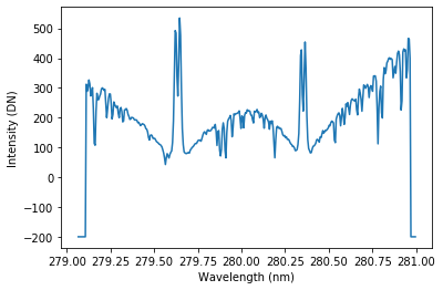
The points at the edges of the plot have a special value of -200 to denote regions not recorded by the detector.
8.2.2.1. Spectroheliograms#
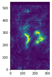
Because in this case we have a 320-step raster, we can use it to build a spectroheliogram at a fixed wavelength position. Suppose we want to do this for the core of the Mg II k line. Its vacuum wavelength is 279.6351 nm, so let’s find the wavelength point closest to this:
>>> mg_index = np.argmin(np.abs(wavelength - 279.6351))
Now we can plot the data with an imshow:
>>> plt.imshow(sp.raster['Mg II k 2796'].data[...,mg_index], vmin=100, vmax=2000)
>>> plt.show()
Let’s go a step farther and, as in the SJI example, make use of astropy.wcs.WCS to get the correct axes when plotting:
>>> figure = plt.figure(figsize=(6, 10))
>>> ax = plt.subplot(projection=wcs.dropaxis(0), slices=('y', 'x'))
>>> ax.set_xlabel("Solar X")
>>> ax.set_ylabel("Solar Y")
>>> ax.imshow(sp.raster['Mg II k 2796'].data[...,mg_index], vmin=100, vmax=2000)
>>> plt.show()
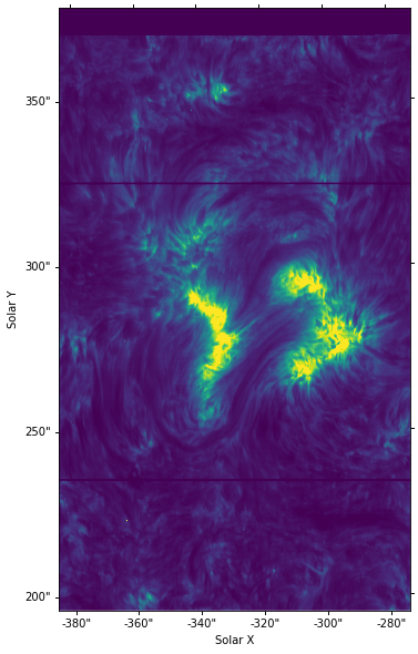
You can compare this image with the ones from the SJI above.
You’ll notice we had to swap the axes in the WCS projection call using slices=('y', 'x') since the rasters are stored in a transposed manner in the FITS files, this has been corrected in the data during extraction.
8.2.2.2. Combining SJI and Raster images#
In the above section we have seen how to load and plot both SJI and raster images. However it can sometimes be very useful to plot these images together on one plot axis. While this may seem trivial, there are some subtleties in both the data structures and WCS that the user should be aware of.
As before we shall start by using astropy.wcs.WCS to create a wcs object for our raster, as well as load in our raster data:
>>> raster_wcs = WCS(extract_irisL2data.getheader(raster_filename, ext=7))
>>> sp = extract_irisL2data.load(raster_filename)
We will also define the wavelength scale and the find the position of the vacuum wavelength of the Mg II k line. We will use this in the plotting of the raster image.
>>> m_to_nm = 1e9  # convert wavelength to nm
>>> nwave = nwave=sp.raster['Mg II k 2796'].data.shape[2]
>>> wavelength = raster_wcs.all_pix2world(np.arange(nwave), [0.], [0.], 0)[0] * m_to_nm
>>> mg_index = np.argmin(np.abs(wavelength - 279.6351))
We will then load in the SJI data and construct a wcs object for the SJI, and load data:
>>> sji_wcs = WCS(extract_irisL2data.only_header(sji_filename, extension=0))
>>> sji = extract_irisL2data.load(sji_filename)
Now, unlike the spectrograph data which have an individual fits file for each raster in the an observation, there is only one fits file for every SJI image in the observation. We therefore need to find the SJI exposure which is closest in time to our raster image. We can find our raster time from the raster header as follows:
>>> raster_time = extract_irisL2data.getheader(raster_filename, ext=0)['DATE_OBS']
The times of each SJI exposure are stored in the date_time_acq key in the loaded SJI data:
>>> sji.SJI['Mg II k 2796']['date_time_acq']
We can now find the closest time corresponding to the raster time, and store the index this occurs at as the variable sji_loctim:
>>> w = min(sji.SJI['Mg II k 2796']['date_time_acq'], key=lambda x: abs(x - raster_time))
>>> sji_loctim = np.where(sji.SJI['Mg II k 2796']['date_time_acq'] == w)[0][0]
As out sji_wcs object is defined from the SJI header, its coordinates (X center, Y center etc.) are defined at the time of the first exposure in the observation.
If the chosen raster is from later in the observation there will be a large difference between the two astropy.wcs.WCS objects, despite the SJI image being from the correct time.
We must therefore find the updated image center coordinates in the sji.SJI object:
>>> x_p, y_p = sji.SJI['SJI_1400']['XCENIX'][sji_loctim]*u.arcsec, sji.SJI['Mg II k 2796']['YCENIX'][sji_loctim]*u.arcsec
>>> xp, yp = u.Quantity(x_p).to(u.deg), u.Quantity(y_p).to(u.deg)
In the preceding code you will notice that we have introduce the use of astropy.units.
We initially define the X-Y centers in arcseconds.
We then convert these in the second line to degrees, as WCS operation are carried out in degrees.
Finally we can create an updated sji_wcs object:
>>> new_sji_wcs = wcs.deepcopy()
>>> new_sji_wcs.wcs.crval[0] = xp.value
>>> new_sji_wcs.wcs.crval[1] = yp.value
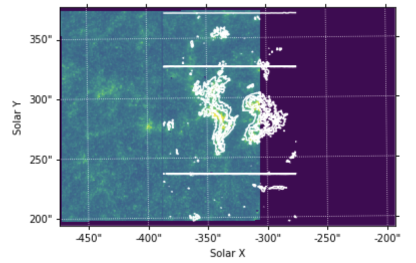
Now we are ready to plot the two data on top of each other.
As with visualizations earlier we need to make use of wcs.dropaxis to remove the time and wavelength axes of the SJI and raster WCS respectively.
>>> notim_raster_wcs  = raster_wcs.dropaxis(0)
>>> ax = plt.subplot(projection=new_sji_wcs.dropaxis(-1))
>>> ax.imshow(sji.SJI['SJI_2796']['data'][:, :, sji_loctim], origin='lower', vmin=-200, vmax=1000, aspect='auto')
>>> ax.contour(sp.raster['Mg II k 2796'].data[..., mg_index], transform=ax.get_transform(notim_raster_wcs.swapaxes(1, 0)), levels=np.arange(100, 2000, 500), colors='white')
>>> ax.set_xlabel("Solar X")
>>> ax.set_ylabel("Solar Y")
8.2.2.3. Time of observations and exposure times#
As in the SJI level 2 files, the exposure times are saved both in the main header and in the auxiliary metadata (as a function of time). In most cases, the exposure times are fixed for all scans in a raster. However, when automatic exposure compensation (AEC) is switched on and there is a very energetic event (e.g. a flare), IRIS will automatically use a lower exposure time to prevent saturation in the detectors. You can see the default exposure time, as well as the maximum and minimum exposure times in the header:
>>> print(hd['EXPTIME'], hd['EXPMIN'], hd['EXPMAX'])
7.99914 7.99909 7.99925
In this case these are all the same, meaning that no change in exposure time took place.
If the exposure time varies, you can get the time-dependent exposure times in seconds from the auxiliary metadata, second to last HDU in the file, after the last line window hd['NWIN']+1.
>>> aux_hd = ei.only_header(raster_filename,extension=hd['NWIN']+1)
>>> aux = ei.only_data(raster_filename,extension=hd['NWIN']+1)
>>> fuv_exptime = aux[:,aux_hd['EXPTIMEF']]
>>> nuv_exptime = aux[:,aux_hd['EXPTIMEN']]
The times of each raster scan are also saved in the auxiliary metadata. These are the time in seconds since the start of the observations, given by:
>>> hd['DATE_OBS']
'2018-01-02T15:31:55.870'
To get an array with the full date/times for individual timesteps, we can make use of numpy.datetime64:
>>> time_diff = aux[:, aux_hd['TIME']]
>>> times = np.datetime64(hd['DATE_OBS']) + time_diff * np.timedelta64(1, 's')