2. Reading IRIS files
The IRIS level 2 FITS files are the standard science data product, and can be read with any standard FITS reader. Here we make use of astropy.io.fits.
For this part we will make use of a dataset from 2018-01-02. Please download the data files and unpack them in your work directory. The commands used here will assume you are at the directory with the IRIS FITS files.
We’ll start by setting up matplotlib and importing the FITS reader. Here we use the inline backend, but for interactive use you should probably use ipympl.
[1]:
%matplotlib inline
import numpy as np
import astropy.io.fits as fits
import matplotlib.pyplot as plt
# Set up some default matplotlib options
plt.rcParams['figure.figsize'] = [10, 6]
plt.rcParams['xtick.direction'] = 'out'
plt.rcParams['image.origin'] = 'lower'
plt.rcParams['image.cmap'] = 'viridis'
2.1. Reading level 2 SJI files
The astropy.io.fits.open function allows one to access both data and header of FITS files. Let us open a SJI file from the 1400 filter. This should be very fast because at this point no data is loaded into memory:
[2]:
sji = fits.open("iris_l2_20180102_153155_3610108077_SJI_1400_t000.fits")
sji
[2]:
[<astropy.io.fits.hdu.image.PrimaryHDU object at 0xa1e46a390>, <astropy.io.fits.hdu.image.ImageHDU object at 0xa1e475b70>, <astropy.io.fits.hdu.table.TableHDU object at 0xa1e483f98>]
In the above you see that a list of three objects is returned: <astropy.io.fits.hdu.image.PrimaryHDU object>, <astropy.io.fits.hdu.image.ImageHDU object>, and <astropy.io.fits.hdu.table.TableHDU object>. The first object contains the science data and header, while the other two contain auxiliary metadata (see ITN 26 on structure of level 2 files).
We can have a look at the main header, which is in the first HDU:
[3]:
sji[0].header
[3]:
SIMPLE  =                    T / Written by IDL:  Tue Mar 20 23:39:27 2018
BITPIX  =                   16 / Number of bits per data pixel
NAXIS   =                    3 / Number of data axes
NAXIS1  =                  845 /
NAXIS2  =                  548 /
NAXIS3  =                   80 /
EXTEND  =                    T / FITS data may contain extensions
DATE    = '2018-03-21'         / Creation UTC (CCCC-MM-DD) date of FITS header
COMMENT FITS (Flexible Image Transport System) format is defined in 'Astronomy
COMMENT and Astrophysics', volume 376, page 359; bibcode 2001A&A...376..359H
TELESCOP= 'IRIS    '           /
INSTRUME= 'SJI     '           /
DATA_LEV=              2.00000 /
LVL_NUM =              2.00000 /
VER_RF2 = 'L12-2017-08-04'     /
DATE_RF2= '2018-03-21T06:00:07.640' /
DATA_SRC=              1.51000 /
ORIGIN  = 'SDO     '           /
BLD_VERS= 'V9R1X   '           /
LUTID   =              0.00000 /
OBSID   = '3610108077'         /
OBS_DESC= 'Very large dense 320-step raster 105.3x175 320s   Deep x 8 Spatial x'
OBSLABEL= '        '           /
OBSTITLE= '        '           /
DATE_OBS= '2018-01-02T15:32:23.340' /
DATE_END= '2018-01-02T16:20:52.740' /
STARTOBS= '2018-01-02T15:31:55.700' /
ENDOBS  = '2018-01-02T16:21:01.960' /
OBSREP  =                    1 /
CAMERA  =                    2 /
STATUS  = 'Quicklook'          /
BTYPE   = 'Intensity'          /
BUNIT   = 'Corrected DN'       /
BSCALE  =                 0.25 /
BZERO   =                 7992 /
HLZ     =                    0 /
SAA     = '           0'       /
SAT_ROT =          0.000227430 /
AECNOBS =                    0 /
AECNRAS =                    0 /
DSUN_OBS=          1.47094E+11 /
IAECEVFL= 'NO      '           /
IAECFLAG= 'NO      '           /
IAECFLFL= 'NO      '           /
TR_MODE = '        '           /
FOVY    =              182.320 /
FOVX    =              281.132 /
XCEN    =             -329.321 /
YCEN    =              286.652 /
SUMSPTRL=                    2 /
SUMSPAT =                    2 /
EXPTIME =              8.00006 /
EXPMIN  =              8.00000 /
EXPMAX  =              8.00011 /
DATAMEAN=              27.0596 /
DATARMS =              21.6273 /
DATAMEDN=              21.8717 /
DATAMIN =             -3219.22 /
DATAMAX =              25706.2 /
DATAVALS=             20441608 /
MISSVALS=             16603192 /
NSATPIX =                    0 /
NSPIKES =                    0 /
TOTVALS =             37044800 /
PERCENTD=              55.1808 /
DATASKEW=              7.27218 /
DATAKURT=              234.259 /
DATAP01 =              8.83011 /
DATAP10 =              12.9206 /
DATAP25 =              16.3524 /
DATAP75 =              31.4368 /
DATAP90 =              46.9377 /
DATAP95 =              61.2195 /
DATAP98 =              81.1593 /
DATAP99 =              97.7437 /
NEXP_PRP=              1.00000 /
NEXP    =                   80 /
NEXPOBS =                  960 /
NRASTERP=                   80 /
RASTYPDX=                    1 /
RASTYPNX=                    1 /
RASRPT  =                    1 /
RASNRPT =                    1 /
CADPL_AV=              36.8290 /
CADPL_DV=              0.00000 /
CADEX_AV=              36.8284 /
CADEX_DV=            0.0124631 /
MISSOBS =                    1 /
MISSRAS =                    0 /
IPRPVER =        1.96000003815 /
IPRPPDBV=        10.0000000000 /
IPRPDVER=             20130925 /
IPRPBVER=             20180310 /
PC1_1   =       0.999970614910 /
PC1_2   =      0.0112785818055 /
PC2_1   =     -0.0112785818055 /
PC2_2   =       0.999970614910 /
PC3_1   =        0.00000000000 /
PC3_2   =        0.00000000000 /
NWIN    =                    1 /
TDET1   = 'SJI     '           /
TDESC1  = 'SJI_1400'           /
TWAVE1  =        1400.00000000 /
TWMIN1  =        1380.00000000 /
TWMAX1  =        1420.00000000 /
TDMEAN1 =              27.0596 /
TDRMS1  =              21.6273 /
TDMEDN1 =              21.8717 /
TDMIN1  =             -3219.22 /
TDMAX1  =              25706.2 /
TDVALS1 =             20441608 /
TMISSV1 =             16603192 /
TSATPX1 =                    0 /
TSPIKE1 =                    0 /
TTOTV1  =             37044800 /
TPCTD1  =              55.1808 /
TDSKEW1 =              7.27218 /
TDKURT1 =              234.259 /
TDP01_1 =              8.83011 /
TDP10_1 =              12.9206 /
TDP25_1 =              16.3524 /
TDP75_1 =              31.4368 /
TDP90_1 =              46.9377 /
TDP95_1 =              61.2195 /
TDP98_1 =              81.1593 /
TDP99_1 =              97.7437 /
TSR1    =                    1 /
TER1    =                  548 /
TSC1    =                    4 /
TEC1    =                  512 /
IPRPFV1 =                  441 /
IPRPGV1 =                    4 /
IPRPPV1 =                  441 /
CDELT1  =             0.332700 /
CDELT2  =             0.332700 /
CDELT3  =              36.8284 /
CRPIX1  =              423.000 /
CRPIX2  =              274.500 /
CRPIX3  =              40.0000 /
CRVAL1  =             -329.321 /
CRVAL2  =              286.652 /
CRVAL3  =              1463.91 /
CTYPE1  = 'HPLN-TAN'           /
CTYPE2  = 'HPLT-TAN'           /
CTYPE3  = 'Time    '           /
CUNIT1  = 'arcsec  '           /
CUNIT2  = 'arcsec  '           /
CUNIT3  = 'seconds '           /
KEYWDDOC= 'http://www.lmsal.com/iris_science/irisfitskeywords.pdf' /
HISTORY iris_prep  Set 1 saturated pixels to Inf
HISTORY iris_prep  Dark v20130925; T=[-59.1,-59.0,-58.3,-59.3,1.4,2.7,2.7,2.7,2.
HISTORY iris_prep  Flat fielded with recnum     440
HISTORY iris_prep  Set permanently bad pixels to 0 prior to warping
HISTORY iris_prep_geowave_roi  ran with rec_num 4
HISTORY iris_prep_geowave_roi  boxwarp set to 1
HISTORY iris_prep_geowave_roi  updated WCS parameters with iris_isp2wcs
HISTORY iris_prep  Used iris_mk_pointdb ver 10
HISTORY iris_prep       Fiducial midpoint shift X,Y [pix]:      0.22    -0.17
HISTORY iris_prep  Used INF_POLY_2D for warping
HISTORY iris_prep VERSION:  1.96
HISTORY iris_prep   ran on 20180321_063639
HISTORY level2  Version L12-2017-08-04
Header entries can be accessed like a dicionary. For example, for the start of the slit-jaw sequence:
[4]:
sji[0].header['STARTOBS']
[4]:
'2018-01-02T15:31:55.700'
The data are saved under sji[0].data. You can see that NAXIS1=845 (spatial x), NAXIS2=548, (spatial y), and NAXIS3=80 (time). Because in Python the arrays are in C order, the dimension order will be reversed:
[5]:
sji[0].data.shape
[5]:
(80, 548, 845)
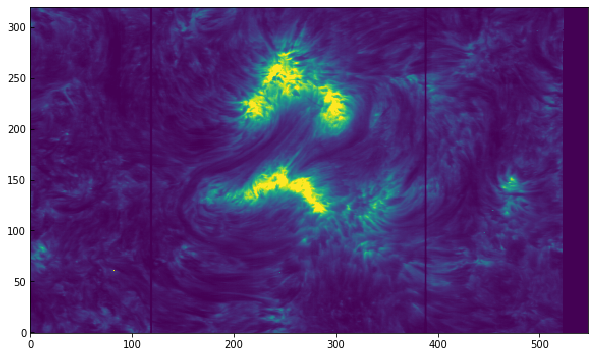
We can plot the first timestep to see how it looks like:
[6]:
plt.imshow(sji[0].data[0])
[6]:
<matplotlib.image.AxesImage at 0xa3545a240>
The image looks washed out because of the automatic scaling. We can get a better scaling by adjusting the maximum and minimum range:
[7]:
plt.imshow(sji[0].data[0], vmin=0, vmax=100)
[7]:
<matplotlib.image.AxesImage at 0xa35ba9390>

In the above, the first time we accessed sji[0].data (or its .shape), the data were loaded into memory, which may take a while depending on your machine. This also means that the data are scaled and have proper DN units.
In some cases, loading the whole data into memory may not be practical or too slow. For these, it is possible to use an approach based on numpy.memmap that allows us to load only parts of the data, and only when necessary. Lets first close the sji object and open it using memmap:
[8]:
sji.close()
sji = fits.open("iris_l2_20180102_153155_3610108077_SJI_1400_t000.fits",
                memmap=True, do_not_scale_image_data=True)
You can still do the operations as before, and the data will only be read when you try to access it, e.g. sji[0].data[0]. Because the IRIS level 2 are saved in the FITS files as 16-bit integers (scaled from 32-bit floating point), this will also use half the memory even if you load the full data into memory. The disadvantage of this procedure is that now the data values are no longer in DN, but in scaled integer units that start at \(-2^{16}/2\). For example, to get the same scaling of
the previous image (from 0 to 100 DNs) we’ll manually scale the frame of interest using the header information:
[9]:
hd = sji[0].header
plt.imshow(sji[0].data[0] * hd['BSCALE'] + hd['BZERO'],
           vmin=0, vmax=100)
[9]:
<matplotlib.image.AxesImage at 0xa1e3d4a20>
2.1.1. Coordinates
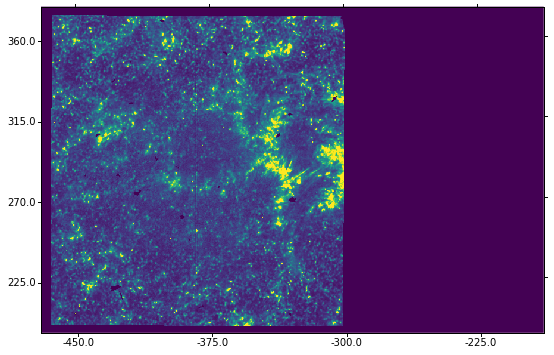
So far, we have used plt.imshow directly, which shows the data in pixel values. Coordinate information is available in the SJI header, with the World Coordinate System (WCS) keywords. The astropy package has an wcs module that allows plotting the image with the proper solar (x, y) coordinates.
First we get the WCS data from the SJI header:
[10]:
from astropy.wcs import WCS
wcs = WCS(hd)
WARNING: FITSFixedWarning: 'unitfix' made the change 'Changed units: 'seconds' -> 's''. [astropy.wcs.wcs]
Inspecting this object we see:
[11]:
wcs
[11]:
WCS Keywords

Number of WCS axes: 3
CTYPE : 'HPLN-TAN'  'HPLT-TAN'  'Time'
CRVAL : -0.09147805555555556  0.07962555555555555  1463.91
CRPIX : 423.0  274.5  40.0
PC1_1 PC1_2 PC1_3  : 0.99997061491  0.0112785818055  0.0
PC2_1 PC2_2 PC2_3  : -0.0112785818055  0.99997061491  0.0
PC3_1 PC3_2 PC3_3  : 0.0  0.0  1.0
CDELT : 9.241666666666666e-05  9.241666666666666e-05  36.8284
NAXIS : 845  548  80
We can see that the first two axes have type of ‘HPLN’ and ‘HPLT’, meaning helioprojective-cartesian longitude and latitude respectively, or solar X and Y. The last axis is time in seconds.
To plot the coordinate axes in matplotlib, we do the following:
[12]:
ax = plt.subplot(projection=wcs.dropaxis(-1))
ax.imshow(sji[0].data[0] * hd['BSCALE'] + hd['BZERO'],
          vmin=0, vmax=100)
[12]:
<matplotlib.image.AxesImage at 0xa35f9ccc0>
We do wcs.dropaxis(-1) because we do not want to plot the time coordinate. The default tickmark scale is in degrees and minutes, but we can convert it to arcsec by changing the coordinate separators to ‘s.ss’:
[13]:
ax = plt.subplot(projection=wcs.dropaxis(-1))
ax.imshow(sji[0].data[0] * hd['BSCALE'] + hd['BZERO'],
          vmin=0, vmax=100)
ax.coords[0].set_major_formatter('s.s')
ax.coords[1].set_major_formatter('s.s')
We can also overplott the coordinates grid by calling ax.grid. For the final figure with grid, we do:
[14]:
ax = plt.subplot(projection=wcs.dropaxis(-1))
ax.imshow(sji[0].data[0] * hd['BSCALE'] + hd['BZERO'],
           vmin=0, vmax=100)
ax.coords[0].set_major_formatter('s.s')
ax.coords[1].set_major_formatter('s.s')
ax.grid(color='w', ls=':')
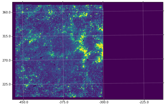
You’ll notice that the solar coordinate grid is slightly tilted from the image axes. This is normal. With different IRIS roll angles, this difference will be even more obvious.
2.1.2. Plotting the slit
We can see the slit in the SJI images, although its position may not be immediately obvious. This is made easier by information in the auxiliary metadata, which is the second FITS HDU. In our example this is in sji[1]:
[15]:
print(sji[1].data.shape)
sji[1].header
(80, 31)
[15]:
XTENSION= 'IMAGE   '           / IMAGE extension
BITPIX  =                  -64 / Number of bits per data pixel
NAXIS   =                    2 / Number of data axes
NAXIS1  =                   31 /
NAXIS2  =                   80 /
PCOUNT  =                    0 / No Group Parameters
GCOUNT  =                    1 / One Data Group
TIME    =                    0 /time of each exposure in s after start of OBS (r
PZTX    =                    1 /PZTX of each exposure in arcsec (rowindex)
PZTY    =                    2 /PZTY of each exposure in arcsec (rowindex)
EXPTIMES=                    3 /SJI Exposure duration of each exposure in s (row
SLTPX1IX=                    4 /Slit center in X of each exposure in window-pixe
SLTPX2IX=                    5 /Slit center in Y of each exposure in window-pixe
SUMSPTRS=                    6 /SJI spectral summing (rowindex)
SUMSPATS=                    7 /SJI spatial summing (rowindex)
DSRCSIX =                    8 /SJI data source level (rowindex)
LUTIDS  =                    9 /SJI LUT ID (rowindex)
XCENIX  =                   10 /XCEN (rowindex)
YCENIX  =                   11 /YCEN (rowindex)
OBS_VRIX=                   12 /Speed of observer in radial direction (rowindex)
OPHASEIX=                   13 /Orbital phase (rowindex)
PC1_1IX =                   14 /PC1_1 (rowindex)
PC1_2IX =                   15 /PC1_2 (rowindex)
PC2_1IX =                   16 /PC2_1 (rowindex)
PC2_2IX =                   17 /PC2_2 (rowindex)
PC3_1IX =                   18 /PC3_1 (rowindex)
PC3_2IX =                   19 /PC3_2 (rowindex)
IT01PSJI=                   20 /SJI PM Temperature (for pointing) (rowindex)
IT06TSJI=                   21 /SJI MidTel Temperature (for pointing) (rowindex)
IT14SSJI=                   22 /SJI Spectrograph +X Temperature (for wavelength)
IT15SSJI=                   23 /SJI Spectrograph +Y Temperature (for wavelength)
IT16SSJI=                   24 /SJI Spectrograph -X Temperature (for wavelength)
IT17SSJI=                   25 /SJI Spectrograph -Y Temperature (for wavelength)
IT18SSJI=                   26 /SJI Spectrograph +Z Temperature (for wavelength)
IT19SSJI=                   27 /SJI Spectrograph -Z Temperature (for wavelength)
POFFXSJI=                   28 /SJI X (spectral direction) shift in pixels (rowi
POFFYSJI=                   29 /SJI Y (spatial direction) shift in pixels (rowin
POFFFSJI=                   30 /SJI Flag indicating source of X and Y offsets (r
The structure of the auxiliary metadata is an array of shape (80, 31). The first axis is the time coordinate, and in the second axis are different variables given by the keys above. For example, SLTPX1IX is the slit’s x pixel coordinate, and is saved in index 4, so sji[1].data[:, 4]. Because this dataset is a raster, the slit position is moving. If we plot an image from the middle sequence, we can overplot the current slit position by using the value of SLTPX1IX:
[16]:
timestep = 40
plt.imshow(sji[0].data[timestep] * hd['BSCALE'] + hd['BZERO'],
           vmin=0, vmax=100)
plt.axvline(x=sji[1].data[timestep, 4], color='black')
[16]:
<matplotlib.lines.Line2D at 0xa35dc4f98>
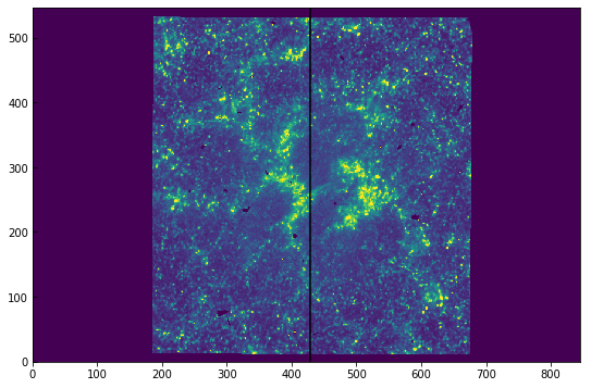
This also works if you have a figure with the WCS coordinates.
2.2. Reading level 2 raster files
IRIS level 2 spectrograph files have a different structure from the SJI files. The main header is similar, but the data are all saved in extension HDUs. The reason for this is that spectrograph level 2 files are organised by spectral windows, which may differ for various observations.
Using the raster file from our example above, we can open the files with astropy.io.fits:
[17]:
from astropy.io import fits
sp = fits.open("iris_l2_20180102_153155_3610108077_raster_t000_r00000.fits")
(The same note about memmap applies as for the SJI files, and is more important in the raster files because they tend to be larger.)
The first FITS HDU has the main header. We can use it to find out what kind of raster this is:
[18]:
hd = sp[0].header
hd['OBS_DESC']
[18]:
'Very large dense 320-step raster 105.3x175 320s Deep x 8 Spatial x'
The number of FITS units in sp is the number of spectral windows plus 3 (with additional metadata). In this case we have 10 FITS units, so 7 spectral windows. We can also look at the NWIN keyword in the main header:
[19]:
print(len(sp))
print(hd['NWIN'])
10
7
Descriptions of the spectral windows, as well as their range in Å, are also saved as header keywords:
[20]:
print('Window. Name      : wave start - wave end\n')
for i in range(hd['NWIN']):
    win = str(i + 1)
    print('{0}. {1:15}: {2:.2f} - {3:.2f} Å'
          ''.format(win, hd['TDESC' + win], hd['TWMIN' + win], hd['TWMAX' + win]))
Window. Name      : wave start - wave end

1. C II 1336      : 1331.77 - 1340.44 Å
2. O I 1356       : 1346.75 - 1357.47 Å
3. Si IV 1394     : 1391.20 - 1396.14 Å
4. Si IV 1403     : 1398.12 - 1406.70 Å
5. 2832           : 2831.34 - 2834.34 Å
6. 2814           : 2812.65 - 2816.47 Å
7. Mg II k 2796   : 2790.65 - 2809.95 Å
Let us work with the Mg II k 2796 window, which is in index 7. The shape of this data array is as follows:
[21]:
sp[7].data.shape
[21]:
(320, 548, 380)
The first axis is the number of raster positions (or time if sit and stare), the second axis the y coordinate (space along slit), and the last axis is the wavelength. We can make use of astropy.wcs to use the WCS header information to convert from pixels to coordinates. For example, for obtaining the wavelength scale we do:
[22]:
from astropy.wcs import WCS
wcs = WCS(sp[7].header)
m_to_nm = 1e9  # convert wavelength to nm
nwave = sp[7].data.shape[2]
wavelength = wcs.all_pix2world(np.arange(nwave), [0.], [0.], 0)[0] * m_to_nm
And we can now plot an example spectrum, say pixel [100, 200]:
[23]:
plt.plot(wavelength, sp[7].data[100, 200])
plt.xlabel("Wavelength (nm)")
plt.ylabel("Intensity (DN)")
[23]:
Text(0,0.5,'Intensity (DN)')
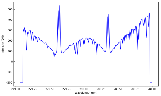
The points at the edges of the plot have a special value of -200 to denote regions not recorded by the detector.
2.2.1. Spectroheliograms
Becase in this case we have a 320-step raster, we can use it to build a spectroheliogram at a fixed wavelength position. Suppose we want to do this for the core of the Mg II k line. Its vacuum wavelength is 279.6351 nm. Let’s find the wavelength point closest to this:
[24]:
mg_index = np.argmin(np.abs(wavelength - 279.6351))
Now we can plot the data with an imshow:
[25]:
plt.imshow(sp[7].data[..., mg_index], vmin=100, vmax=2000)
[25]:
<matplotlib.image.AxesImage at 0xa379d6ac8>
The two dark fiducial lines appear as vertical lines, so we can infer that the raster scanned in the y direction. This was a zero roll observation, so to have the axis roughly aligned with solar X and Y we should instead plot the transpose of the data, e.g., sp[7].data[..., mg_index].T. But let’s go a step farther and, as in the SJI example, make use of astropy.wcs to get the correct axes when plotting:
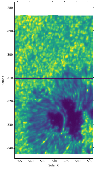
[26]:
figure = plt.figure(figsize=(6, 10))
ax = plt.subplot(projection=wcs.dropaxis(0), slices=('y', 'x'))
ax.imshow(sp[7].data[..., mg_index].T, vmin=100, vmax=2000)
ax.coords[0].set_major_formatter('s.s')
ax.coords[1].set_major_formatter('s.s')
ax.set_xlabel("Solar X")
ax.set_ylabel("Solar Y")
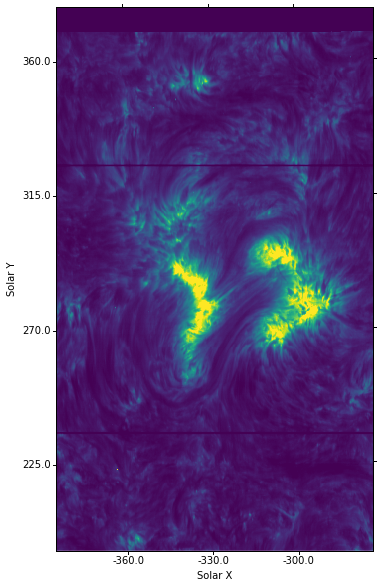
You can compare this image with the ones from the SJI above.
You’ll notice that besides using the transposed data, sp[7].data[..., mg_index].T, we also had to swap the axes in the WCS projection call using slices=('y', 'x').
2.2.2. Time of observations and exposure times
As in the SJI level 2 files, the exposure times are saved both in the main header and in the auxiliary metadata (as a function of time). In most cases, the exposure times are fixed for all scans in a raster. However, when automatic exposure compensation (AEC) is switched on and there is a very energetic event (e.g. a flare), IRIS will automatically use a lower exposure time to prevent saturation in the detectors. You can see the default exposure time, as well as the maximum and minimum exposure times in the header:
[27]:
print(hd['EXPTIME'], hd['EXPMIN'], hd['EXPMAX'])
7.99914 7.99909 7.99925
In this case these are all the same, meaning that no change in exposure time took place.
If the exposure time varies, you can get the time-dependent exposure times in seconds from the auxiliary metadata, second to last HDU in the file:
[28]:
fuv_exptime = sp[-2].data[:, sp[-2].header['EXPTIMEF']]
nuv_exptime = sp[-2].data[:, sp[-2].header['EXPTIMEN']]
The times of each raster scan are also saved in the auxiliary metadata, under sp[-2].data[:, 0]. These are the time in seconds since the start of the observations, given by
[29]:
hd['DATE_OBS']
[29]:
'2018-01-02T15:31:55.870'
To get an array with the full date/times for individual timesteps, we can make use of numpy.datetime64:
[30]:
time_diff = sp[-2].data[:, sp[-2].header['TIME']]
times = np.datetime64(hd['DATE_OBS']) + time_diff * np.timedelta64(1, 's')
2.3. Reading level 3 files
IRIS level 3 FITS files combine several spectrograph raster files into two files. They combine the temporal domain into raster data, resulting in 4-D arrays of dimensions (nx, ny, nwave, ntime). The main application of level 3 files is the CRISPEX data analysis software. Level 3 files are not available for download, and the users are expected to create them by combining level 2 spectrograph files.
To date, there is no Python tool to create level 3 files, so all level 3 files analysed here must be created with IDL.
In this example we will work with a level 3 file created from the observation 20161012_073017_3620256863.
Level 3 files can include all wavelength windows in level 2 files, or just a subset. Here we work on an example with all wavelength windows. We can open the FITS file in the same way as level 2 files:
[31]:
data = fits.open("iris_l3_20161012_073017_3620256863_t000_all_im.fits",
                 memmap=True)
len(data)
[31]:
4
We confirm that the file has 4 FITS HDUs. They contain, in order: main data, wavelength scale, time of observation, and location of slit in slit-jaw images.
We make use of memmap=True to save memory. Level 3 data are saved as 32-bit floating point, and unlike level 2 files, there is no FITS scaling. This means that we’ll get the values in data number (DN) even using memmap.
The main header of level 3 files is stored in the first HDU. Its keywords are similar to level 2 keywords, with some small differences. In level 3 files, the wavelength axis concatenates all spectral windows, but information about each window is stored in the header. Keyword NWIN again specifies the number of wavelength windows, while WSTARTn, WWIDTHn, WDESCn represent respectively the starting wavelength index, the number of wavelength points, and a description for wavelength
window n. We can print out a summary table with:
[32]:
hd = data[0].header
print('Window. Name      : central wavelength, wave start , wavelength points\n')
for i in range(hd['NWIN']):
    win = str(i + 1)
    print('{0}. {1:15}: {2:.2f} Å , {3} , {4}'
          ''.format(win, hd['WDESC' + win], hd['TWAVE' + win],
                    hd['WSTART' + win], hd['WWIDTH' + win]))
Window. Name      : central wavelength, wave start , wavelength points

1. C II 1336      : 1335.71 Å , 0 , 182
2. Fe XII 1349    : 1349.43 Å , 182 , 117
3. O I 1356       : 1355.60 Å , 299 , 166
4. Si IV 1394     : 1393.78 Å , 465 , 199
5. Si IV 1403     : 1402.77 Å , 664 , 295
6. 2832           : 2832.88 Å , 959 , 103
7. 2814           : 2814.61 Å , 1062 , 136
8. Mg II k 2796   : 2796.20 Å , 1198 , 521
The main data has dimensions of 'x' 'y' 'wave' 'time', where x is the raster direction, y is the direction along the slit, wave is wavelength points, and time is the number of raster scans. In Python, because of C-order loading, the dimensions are reversed and the shape of the data is (time, wave, y, x). In this example:
[33]:
data[0].data.shape
[33]:
(14, 1719, 402, 96)
In this example you can also notice that the wavelength windows do not have to be monotonic.
The wavelength and time arrays are saved in the first and second extensions, respectively. We can get them by doing:
[34]:
wavelength = data[1].data / 10.  # convert from Å to nm
times = np.datetime64(hd['DATE_OBS']) + data[2].data * np.timedelta64(1, 's')
Here times is a 2D array with shape of (time, x) because each raster step occurs at a different time.
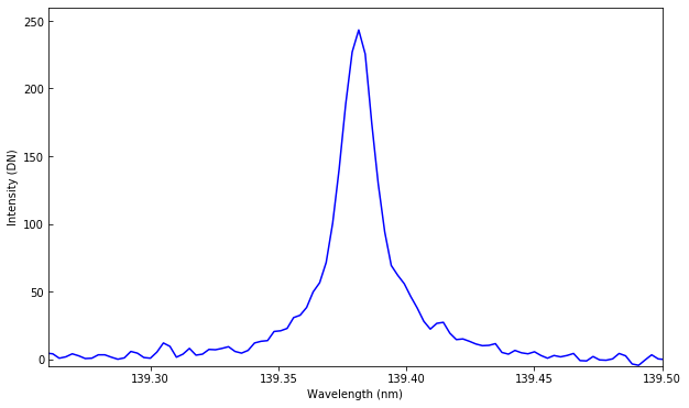
We can plot the spectrum at a single point in the raster, eg. x=93, y=131:
[35]:
plt.plot(wavelength, data[0].data[5, :, 131, 93])
plt.axis([139.26, 139.5, -5, 260])  # zoom to Si IV 139.39 line
plt.xlabel("Wavelength (nm)")
plt.ylabel("Intensity (DN)")
[35]:
Text(0,0.5,'Intensity (DN)')
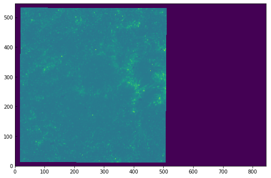
We can also plot a spectroheliogram at a specific wavelength. E.g., in the NUV continuum, first scan:
[36]:
# index of wavelength in continuum at 283.2 nm
cont_wave = np.argmin(np.abs(wavelength - 283.2))
aspect_ratio = hd['CDELT2'] / hd['CDELT1']
fig = plt.figure(figsize=(6, 10))
plt.imshow(data[0].data[0, cont_wave], vmin=0, vmax=250,
           aspect=aspect_ratio)
[36]:
<matplotlib.image.AxesImage at 0xa37ac3c88>
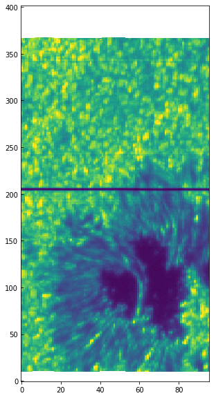
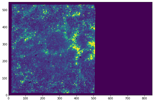
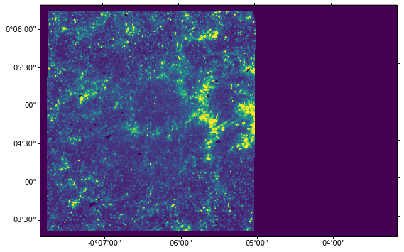
We use the aspect keyword with the ratio of y pixel size to x pixel size because the resolution in the scanning direction (x) is about half of the resolution along the slit (y). We can use astropy.wcs and the header information to properly plot the spectroheliogram in solar X, Y coordinates:
[37]:
from astropy.wcs import WCS
wcs = WCS(data[0].header)
fig = plt.figure(figsize=(6, 10))
ax = plt.subplot(projection=wcs.dropaxis(-1).dropaxis(-1))
img = ax.imshow(data[0].data[0, cont_wave], vmin=0, vmax=250,
          aspect=aspect_ratio)
ax.set_xlabel("Solar X")
ax.set_ylabel("Solar Y")
Here we drop the last two WCS axes (wavelength and time). Notice that here the coordinates already appear in arcsec unlike in the level 2 case (this is because the WCS header format is slightly different).
With IPython and matplotlib, we can make an animation of the spectroheliogram by scanning in wavelength. An example for the Mg II h line:
[38]:
from matplotlib import animation
from IPython.display import HTML

blue_wing = np.argmin(np.abs(wavelength - 280.15))
red_wing = np.argmin(np.abs(wavelength - 280.55))
npts = red_wing - blue_wing
img.norm.vmin = 0

def init():
    ax.set_title('%.2f nm' % wavelength[blue_wing])
    img.norm.vmax = 40
    img.set_data(data[0].data[0, blue_wing])
    return (img,)

def animate(i):
    tmp = data[0].data[0, blue_wing + i]
    img.norm.vmax = np.nanmedian(tmp) * 2
    ax.set_title('%.2f nm' % wavelength[blue_wing + i])
    img.set_data(tmp)
    return (img,)

anim = animation.FuncAnimation(fig, animate, init_func=init,
                               frames=npts, interval=40, blit=True)
HTML(anim.to_html5_video())
[38]:
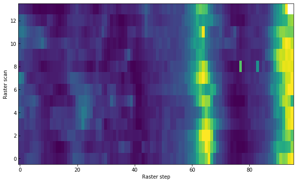
Another way to plot the data is to look at the time domain. For example, at the core of the Mg II k line at x=70:
[39]:
mg_index = np.argmin(np.abs(wavelength - 279.6351))
plt.imshow(data[0].data[:, mg_index, 70], vmin=100, vmax=450, aspect='auto')
plt.xlabel("Raster step")
plt.ylabel("Raster scan")
[39]:
Text(0,0.5,'Raster scan')