Spectral line fitting
Contents
4. Spectral line fitting#
As IRIS is an imaging spectrometer, aside from it’s imaging data products, detailed observations of spectral lines are also acquired. These spectral lines, when analyzed can provide a wealth of information about the solar atmosphere. A key tool in the analysis process is spectral line fitting. This is the process by which we can quantify the shape of the spectral line mathematically, and subsequently use these fits to calculate various physical parameters which help to explain the composition and dynamics of the solar atmosphere.
To this end iris_lmsalpy contains the iris_fit module.
This module provides several functions that allow the user to fit spectral lines observed by IRIS, and then utilize these fits to derive physical parameters from them.
This document will outline the basic functionality of iris_fit through worked examples.
Warning
iris_fit is currently under continued development, and as such is liable to change.
4.1. Fitting Spectra#
As stated, the primary purpose of this module is to fit the various spectral lines observed by IRIS.
To do this iris_fit has several functions for the user to choose from.
Before detailing how to use these, we first need spectra to fit.
As in Section 8 we will be using the dataset from 2018-01-02.
We will first import some packages that we will be using:
>>> import numpy as np
>>> from iris_lmsalpy import fit_iris
>>> import iris_lmsalpy.extract_irisL2data as ei
We will then load in our IRIS data and check to see what lines it contains.
>>> lines = ei.show_lines(raster_filename)
Extracting information from file /iris_l2_20180102_153155_3610108077_raster_t000_r00000.fits...

Available data with size Y x X x Wavelength are stored in windows labeled as:

--------------------------------------------------------------------
Index --- Window label --- Y x X x WL --- Spectral range [AA] (band)
--------------------------------------------------------------------
  0          C II 1336         548x320x335     1331.77 - 1340.44  (FUV)
  1          O I 1356          548x320x413     1346.75 - 1357.44  (FUV)
  2          Si IV 1394        548x320x194     1391.20 - 1396.11  (FUV)
  3          Si IV 1403        548x320x337     1398.12 - 1406.67  (FUV)
  4          2832              548x320x60      2831.34 - 2834.34  (NUV)
  5          2814              548x320x76      2812.65 - 2816.47  (NUV)
  6          Mg II k 2796      548x320x380     2790.65 - 2809.95  (NUV)
--------------------------------------------------------------------

Observation description:  Very large dense 320-step raster 105.3x175 320s   Deep x 8 Spatial x
We now want to load in the Si IV 1403 and Mg II 2796 wavelength windows. For this particular observation, these are windows 3 and 6 respectively:
>>> sp = ei.load(raster_filename, window_info=[lines[3], lines[6]], verbose=True)

The provided file is a raster IRIS Level 2 data file.

Extracting information from file /iris_l2_20180102_153155_3610108077_raster_t000_r00000.fits...

Available data with size Y x X x Wavelength are stored in windows labeled as:

--------------------------------------------------------------------
Index --- Window label --- Y x X x WL --- Spectral range [AA] (band)
--------------------------------------------------------------------
  0          C II 1336         548x320x335     1331.77 - 1340.44  (FUV)
  1          O I 1356          548x320x413     1346.75 - 1357.44  (FUV)
  2          Si IV 1394        548x320x194     1391.20 - 1396.11  (FUV)
  3          Si IV 1403        548x320x337     1398.12 - 1406.67  (FUV)
  4          2832              548x320x60      2831.34 - 2834.34  (NUV)
  5          2814              548x320x76      2812.65 - 2816.47  (NUV)
  6          Mg II k 2796      548x320x380     2790.65 - 2809.95  (NUV)
--------------------------------------------------------------------

Observation description:  Very large dense 320-step raster 105.3x175 320s   Deep x 8 Spatial x

Creating temporary file...  /var/folders/zp/92y232y95xnfm5d2nr8mcbdh0000gn/T/tmptxpnky88
Creating temporary file...  /var/folders/zp/92y232y95xnfm5d2nr8mcbdh0000gn/T/tmptwjmyq_b
The selected data are passed to the output variable (e.g., iris_raster) as a dictionary with the following entries:
iris_raster.raster['Si IV 1403']iris_raster.raster['Mg II k 2796']
iris_fit has three in-build function for fitting, which make use of several SciPy modules.
The three fitting function we present are fit_siiv, fit_mgii and fit_gen.
As two of the most commonly studied lines IRIS observes are Si IV 1403 and Mg II k 2796, fit_siiv and fit_mgii are designed to have several default options for commonly used fits.
4.1.1. fit_siiv#
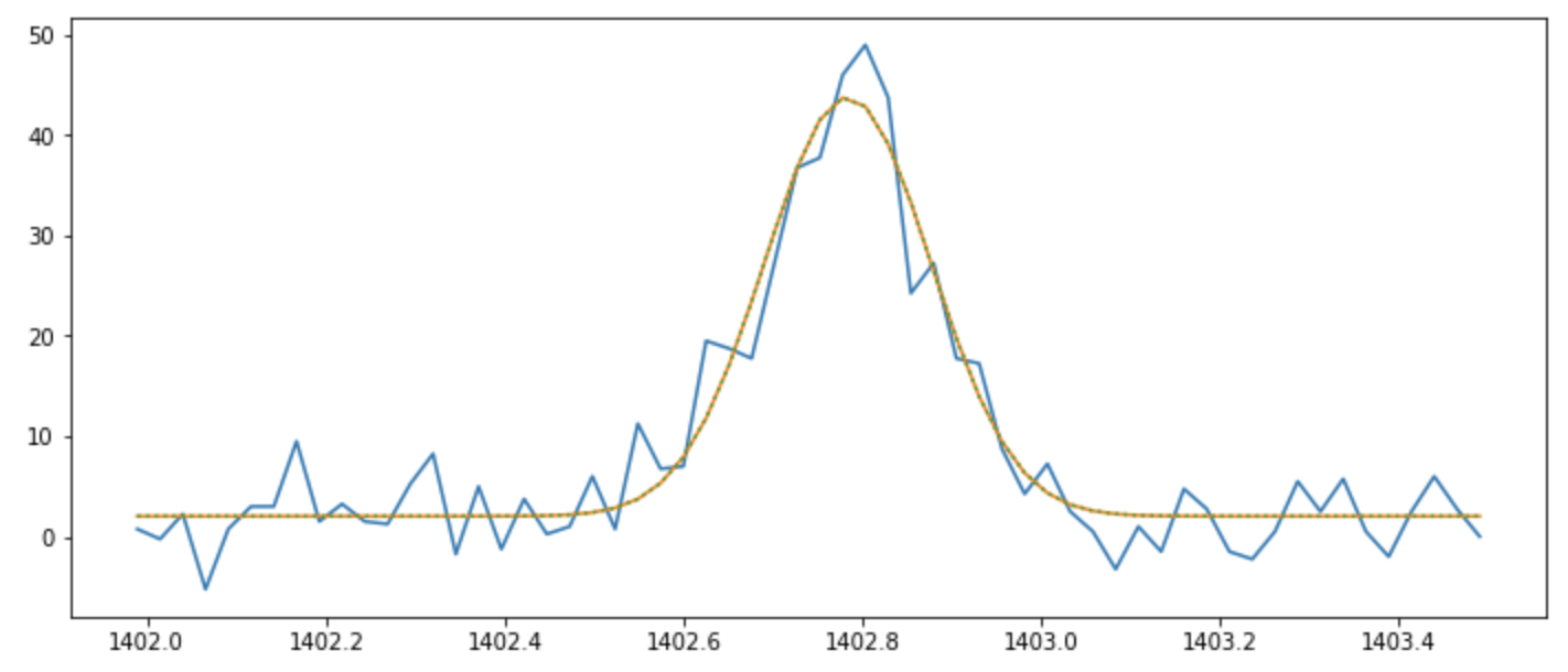
We will first look at how to use fit_siiv.
This function takes a spectra and its corresponding wavelength array and by default will fit a single Gaussian profile to the line and will also plot the results of the fitting.
The function returns four quantities:
The fitted line profile
A list of fitted Gaussians (if fitting a single Gaussian this will be the same as the fitted profile)
The parameters that define the fitted profiles
The errors associated with these parameters.
>>> si_iris_fit, si_list_gauss, si_best_val, si_errors = fit_iris.fit_siiv(sp.raster[lines[3]]['data'][300, 90, :], sp.raster[lines[3]]['wl'])
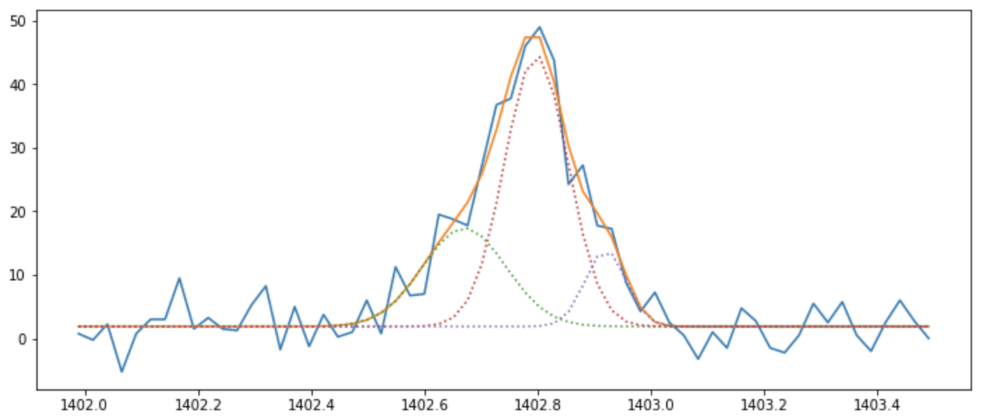
The keywords two and three can be used to fit two or three Gaussians to the spectral line e.g.,
>>> si_iris_fit, si_list_gauss, si_best_val, si_errors = fit_iris.fit_siiv(sp.raster[lines[3]]['data'][300, 90, :], sp.raster[lines[3]]['wl'], three=True)
If more than three Gaussains are desired or the default parameters and limits of the fits need to be changed, this can be achieved keywords and keyword arguments. A full list of these keywords and keyword arguments can be accessed by typing the following:
>>> help(iris_fit.fit_siiv)
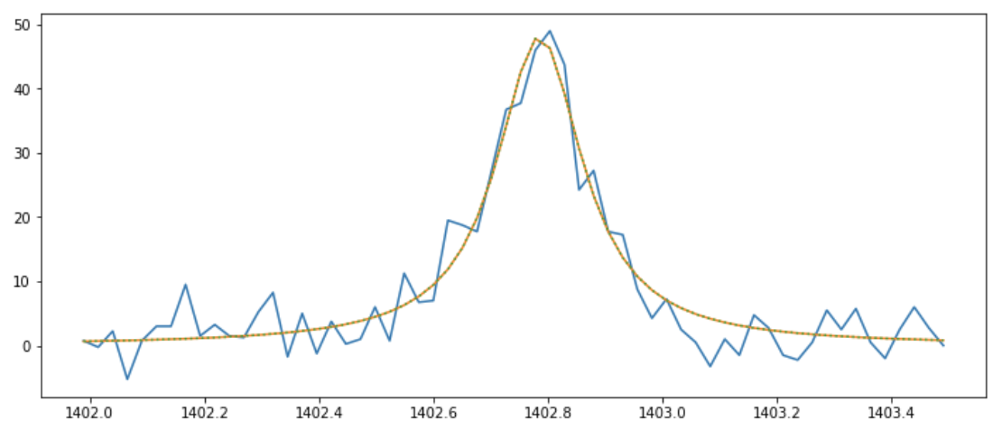
Sometimes, a Gaussain (or Gaussians) is not the most appropriate distribution to fit the observed line.
fit_siiv therefore contains the lorentz keyword.
When set, this keyword will fit a single Lorentzian distribution to the inputted spectra.
>>> si_iris_fit, si_list_gauss, si_best_val, si_errors = fit_iris.fit_siiv(sp.raster[lines[3]]['data'][300, 90, :], sp.raster[lines[3]]['wl'], lorentz=True)
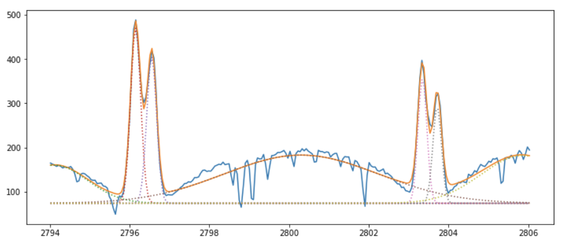
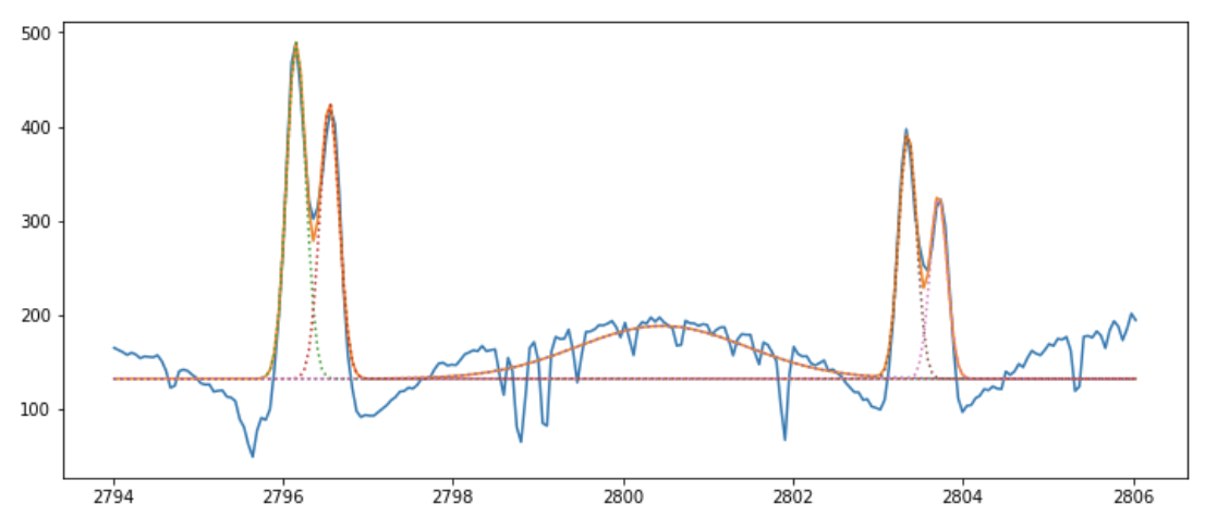
4.1.2. fit_mgii#
The function fit_mgii is very similar to fit_siiv in its workings.
This function takes an input Mg II spectra and its corresponding wavelength array and by default will fit 7 Gaussian profiles to the line, and will also plot the results of the fitting.
The function returns four quantities:
The fitted line profile
A list of fitted Gaussians
The parameters that define the fitted profiles
The errors associated with these parameters.
>>> mg_iris_fit, mg_list_gauss, mg_best_val, mg_errors = fit_iris.fit_mgii(sp.raster[lines[6]]['data'][300, 90, :], sp.raster[lines[6]]['wl'])
The keywords four and five can be used to fit four or five Gaussians to the spectral line e.g.,
>>> mg_iris_fit, mg_list_gauss, mg_best_val, mg_errors = fit_iris.fit_mgii(sp.raster[lines[6]]['data'][300, 90, :], sp.raster[lines[6]]['wl'], five=True)
If more than three Gaussains are desired or the default parameters and limits of the fits need to be changed, this can be achieved keywords and keyword arguments. A full list of these keywords and keyword arguments can be accessed by typing the following:
>>> help(iris_fit.fit_mgii)
4.1.3. fit_gen#
Of course, IRIS observes many more spectral lines than just Si IV and Mg II.
As such, we provide the function fit_gen, which can be applied to any given line observed by IRIS.
As before this function by default fits Gaussian profiles, but Lorentzians can be used by selecting the keyword lorentz.
However, unlike the previous two functions, default parameters, limits and wavelength range must be defined by the user.
These parameters are as follows:
init_vals : `list`
    With parameters c, amp1, mu1, sigma1,... ampN, muN, sigmaN,
                    with c as offset constant in Y.

    For a Lorenzian distribution these parameters are c, amp1, x0_1,
    gamma1, ... ampN, x0_N, gammaN, with:

        c     =  offset constant in Y.
        amp   = amplitude of the profile
        x0    = location parameter
        gamma = half-width at half maximum

limits: 2xN `list`
    Upper and lower limits.

wl_range: `list`
    Min and max wavelength over which corresponding to ``init_vals``.
    Fitting is carried out in Angstrom (Å).
4.2. Derived Quantities#
The fit_iris module as contains functions that take the results of the fitting and return various derived physical quantities of the observed plasma.
4.2.1. Non-thermal velocity#
An important quantity used in the analysis of observed spectral lines is know non-thermal velocity or non-thermal line width.
All spectral lines have a thermal (Maxwellian) line width that is defined by quantum mechanics.
However, observed spectral lines often have widths larger than these thermal widths.
A portion of this additional width is due to the spectrometer, which we denote as instrumental line width (inst_wid) in the function.
The remainder of the observed width of the spectral line, once thermal and instrumental width have been subtracted, is deemed to be the “non-thermal width”.
To allow the calculation we provide the function iris_vnt.
It allows for the calculation of the non-thermal velocity, via the calculation of the corresponding thermal width for the ion understudy.
As an example we will use the single Gaussian fit form earlier in this tutorial.
We must first convert the sigma quantity, the standard deviation, of the fitted Gaussian into Full Width Half Maximum (FWHM).
si_fwhm = 2.355 * si_best_val[3]
Then we can use the instrumental width for IRIS and the iris_vnt function to calculate the non-thermal velocity.
v_nt = iris_vnt('Si', 'iv', 1402.77, si_fwhm ,inst_wid=0.0286, verbose=True)
Note
IRIS has two wavelength windows, FUV short and FUV long. These both have different instrumental FWHM. These are:
FUV short = 0.0286Å
FUV long = 0.0318Å