3. Visualizing IRIS Level 2 data

3.1. IRIS Level 2 SJI data

We have developed a visualization tool to display the SJI data contained in the SoI object. Indeed, the object SoI was built to be easily displayed by this and other functions. The visualization tool is a method of the ei.SJI class, and it accepts a SoI as an input:

# Let's visualize the SJI data
>>> ei.SJI.quick_look(iris_sji)
# or cleaner
>>> vis = ei.SJI.quick_look
>>> vis(iris_sji)

Because iris_sji is a SoI, i.e. an object of the ei.SJI class, we can simply use:

>>> iris_sji.quick_look()

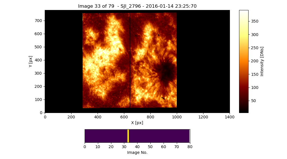
Fig. 3.1 The output of the iris_sji.SJI.quick_look method applied to the SoI object named iris_sji, which contains data from the IRIS spectral window “SJI_2796”.

Fig. 3.1 shows the result of the previous command. The bottom panel allows us to move backward and forward the selected position in the \(3^{rd}\) dimension of the data cube by hovering the mouse over this panel.

The SoI object has an attribute that sets the lower and upper limits of the image displayed by the ei.SJI.quick_look method. These limits are automatically calculated by the code when the SoI is built. The user can change these values, which may be useful for a better visualization manually:

>>> print(iris_sji.SJI['SJI_2796'].clip_ima)
[5, 1031.3840103149414]
>>> iris_sji.SJI['SJI_2796'].clip_ima = [30, 500]
>>> iris_sji.quick_look()

or dynamically when the visualization window has been displayed by pressing the keys “u/i/o/p” (see below).

The ei.SJI.quick_look method, or iris_sji.quick_look in our example, allow us to inspect interactively the data stored in the iris_sji.SJI['SJI_2796'].data attribute. The data dimensions are “[Y, X, time_step]”: - “Y” being the direction along the slit - “X” the direction perpendicular to the slit or the steps used to sample the solar surface perpendicularly to the slit either temporally (sit-and-stare) or spatially - “time_step”, a time of the acquisition taken during the observation.

iris_sji.quick_look method uses matplotlib to display the images, we can take advantage of the options provided by that package. Thus, we can use the zoom option to visualize and animate the SJI data (see Fig. 3.2). Note that the bottom panel has been also zoomed-in. That allows us to make a “mini-loop animation” in those steps of our interest, in the example, between the image 30 to 55. We can recover the full access to all the images by pressing “h”.

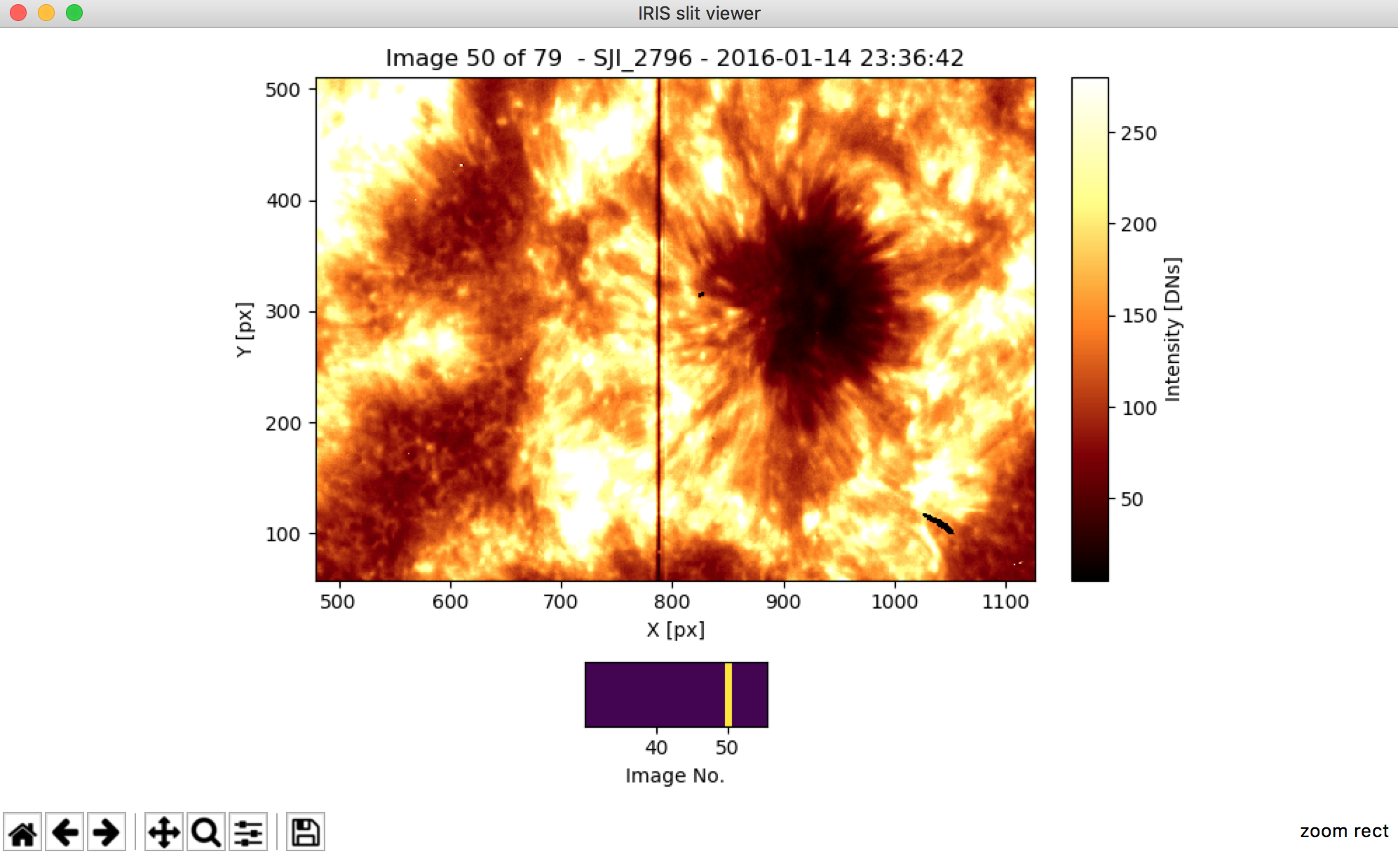
Fig. 3.2 The output of the iris_sji.SJI['SJI_2796'].quick_look() zoomed in by using the zoom option provided by matplotlib. By clicking in the magnifier icon, the \(5^{th}\) icon in the lower left corner. Note that zooming-in in the bottom panel allows us to make “mini-loop animation”.

We have developed and integrated new functionalities to the matplotlib figure. These new functions are controlled by some shortcut keys that are summarized in the following list and in the Fig. 3.3. They allow us to:

• Space bar: start/stop the animation of displaying the data corresponding to the steps in the \(3^{rd}\) dimension.

• -/+: controls the speed of the SJI animation. By pressing -/+ the animation is displayed slower/faster.

• Left/right arrow: allows to move backward/forward step-by-step along the \(3^{rd}\) dimension.

• v/V: show/hide a dashed vertical line over the slit, by pressing V, the plotted line is thicker.

• H: returns to the initial display parameters. This affects the image displayed (e.g. after being zoomed-in) and to the contrast intensity levels of the image.

• u/i/o/p: these keys are used to control the contrast intensity of the image displayed in the figure. By pressing u/i the lower limit of the intensity image is decreased/increased respectively. By pressing o/p, the higher limit of the intensity image is decreased/increased respectively. If one of the limits is 0, these keys will not have an effect on that limit. In this case, it may be convenient to change this value in the attribute iris_sji.SJI[window_label].clip_ima, as it has been done above.

• a: add a Point of IRIS or PoI to the SoI. Thus, the user can store a particular slit acquisition. Note that a PoI contains the data values for a given step, i.e. the 2D data corresponding to the plane [Y,X,selected_step], and some relevant information for the display.

• e/r/t: these keys allow us to erase, return or go to a saved PoI.

• ? or /: show help menu.

• q: quit the visualization tool.

These keys - except e/r/t - and the native matplotlib capabilities can be used during the animation mode. We have to be especially careful when the animation is working to not continuously press the control keys, e.g., the contrast intensity control keys u/i/o/p, and wait any time the keys are pressed. That allows to the animation loop to keep the control on the figure. We can always stop the animation, adjust the configuration of the display, and restart the animation.

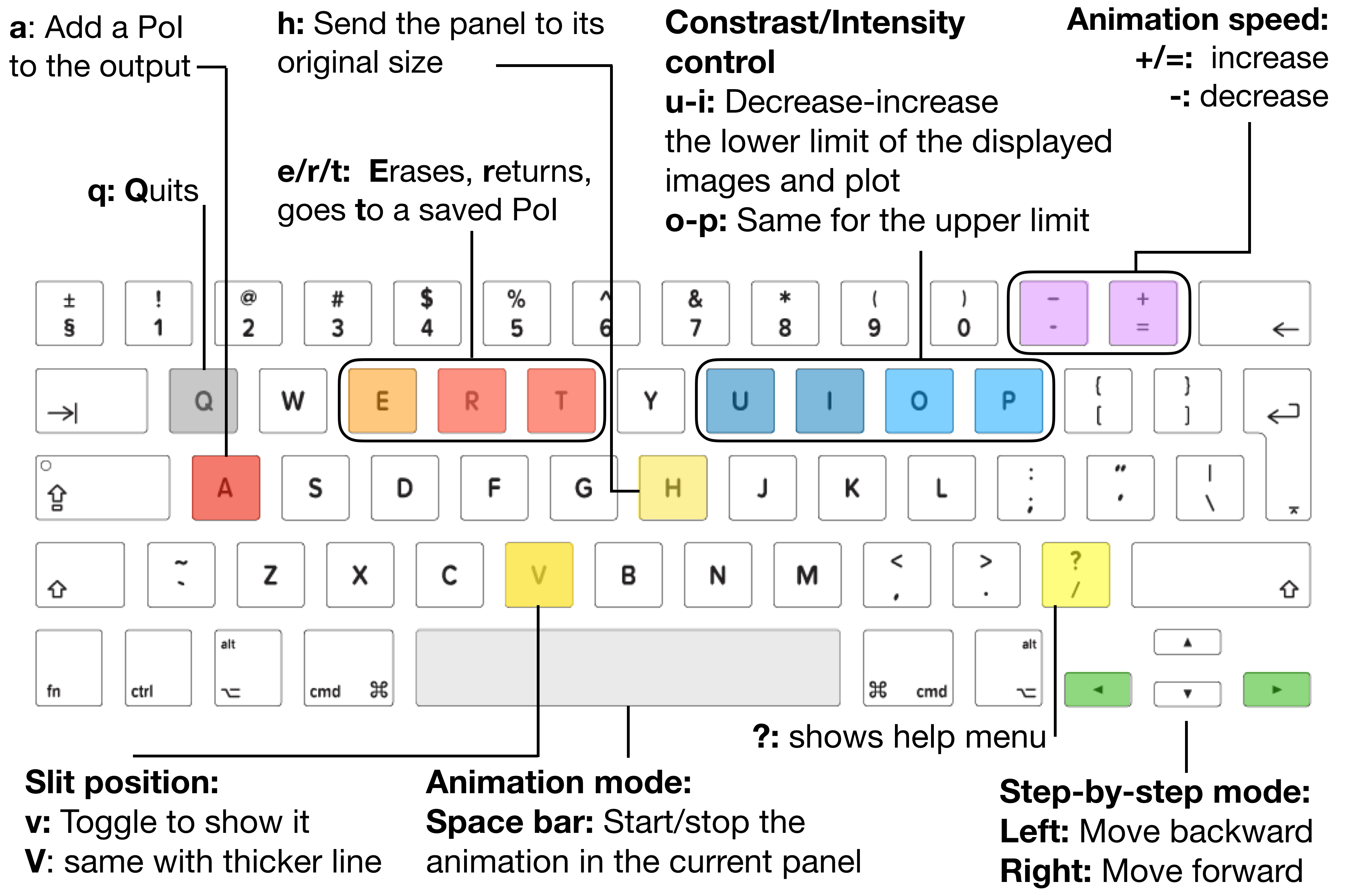
Fig. 3.3 Shortcut keys to inspect SJI IRIS Level 2 data with the visualization tool ei.SJI.quick_look.

The performance of the animation mode is limited by the data size and the user’s computer features, but mostly by the capabilities of matplotlib package, which was not designed to visualize animations. A faster solution can be found in Section 6.

3.2. IRIS Level 2 raster data

We can visualize the data stored in a key corresponding to a spectral window using the method ei.raster.quick_look, or directly from this method in the RoI object. Thus, to visualize the data in the “Mg II k 2796” spectral window contained in the RoI called iris_raster in our example, we use:

# Let's visualize the data in the spectral window ``Mg II k 2796``
>>> iris_raster.quick_look()

Fig. 3.4 shows the output of the iris_raster.quick_look() method. Three panels are shown:

1. In the upper left panel, the spatial distribution of intensity for a given spectral position with the title “XY map” at a wavelength given in Angstrom and in the data cube position (\(3^{rd}\) dimension)`

2. In the upper right panel, the full spectra along the slit for a given sampling step (either spatial or temporal) with the title “Slit spectra” at the position in the “XY map” and in the data cube (\(2 {nd}\) dimension). The bottom panel, titled “Spectra”, shows the spectral distribution at the “[X,Y]” position of the “XY” map, which also corresponds to the intensity along the “X” direction (wavelength in pixels) at the “Y” position (along the slit) of the “Slit spectra” panel.

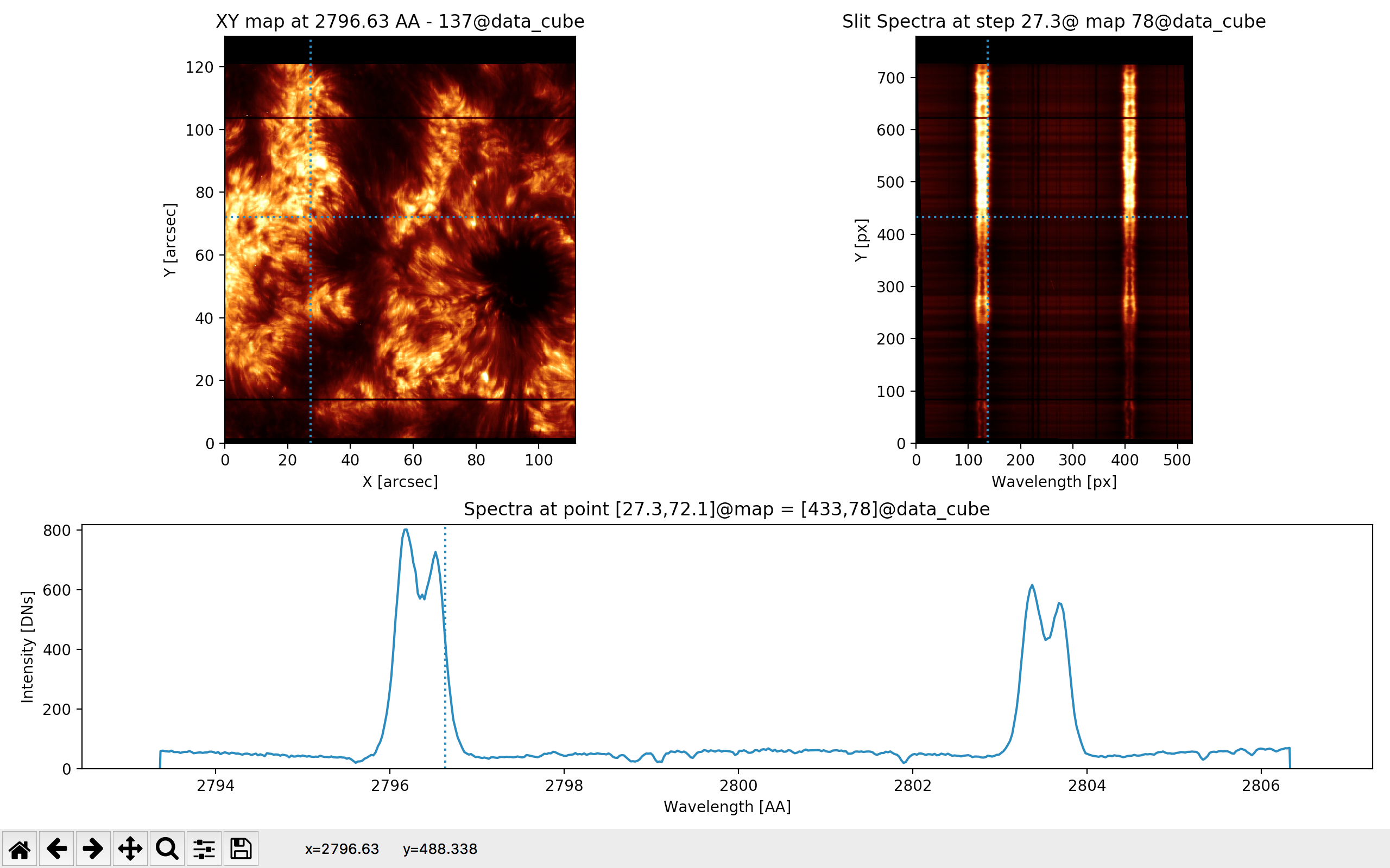
Fig. 3.4 The output of the quick_look method of the RoI called iris_raster, i.e., of iris_raster.quick_look().

The three panels are dynamically connected, which means that the movement of the mouse in one panel has an impact on the others and their titles. This may make the inspection of the data a bit slow, depending of the size of the data and the hardware features of the user’s machine.

Again, as we are using matplotlib package, we can use its options, e.g., to save the image displayed we can type s to save the current figure, or use the zoom option to look in detail an interesting region.

When a panel is zoomed-in, the user can automatically matches the axes shared with other panels. Thus, if we zoom in the “Slit spectra”, we change the region shown both in the axis corresponding to the Slit (axis “Y” in the “XY map” panel) and in the axis corresponding to the wavelengths (axis “X” in the “Spectra”). The user can automatically fits sharing axes by pressing v.

One of the most useful capabilities of the visualization tool is the ability to easily show several spectral windows stored in a RoI. The following commands load and store 4 spectral regions in a RoI, which are visualized with iris_raster.quick_look.

# Let's check again the available spectral windows that we stored
# in the 'lines' variable
>>> for j, i in enumerate(lines): print(j, i)
0 C II 1336
1 Fe XII 1349
2 O I 1356
3 Si IV 1394
4 Si IV 1403
5 2832
6 2814
7 Mg II k 2796

# Let's load 4 spectral windows of out interest
>>> iris_raster = ei.load(raster_filename, window_info = lines[[0,3,5,7]])

# Let's visualize the 4 spectral windows
>>> ei.raster.quick_look(iris_raster)

The way to go backward/forward from a spectral window to another is by pressing n/m. Note that the panels for the different spectral windows are independently considered. Thus, for instance, we can zoom-in in the “XY map” panel for the window showing the data of “Mg II k 2796” and not in the others, or change the contrast intensity in just the “Si IV 1394” panels. Of course, we can be interested in to inspect in detail a particular region in all the selected spectral windows. After, zoomed in that region of interest in the “XY map” of a particular spectral window, if we press N/M we will move backward/forward through the spectral windows showing always the same region in the “XY map” panel. The animation in Fig. 3.5 shows how this looks when the we inspect the same zoomed-in area in all the selected spectral windows by pressing N/M.

Fig. 3.5 Inspecting simultaneously several spectral windows with the iris_raster.quick_look() method. iris_raster is a RoI that, in addition to the quick_look methods, contains data of “C II 1336”, “Si IV 1394”, “2832”, and “Mg II k 2796” spectra. Note that the “Y” axis of the “SlitSpectra” has been automatically fit to the slit portion zoomed-in in the “XY map” by pressing v when the mouse was on this last panel.

As the raster IRIS data might be very different in their spatial or temporal dimensions, e.g., a raster scan over an active region or a sit-and-stare observation during 1h, the visualization code allows to choose between several combinations of spatial/temporal scales by pressing y. By default ei.raster.quick_look uses that ratio of the scales in the “X” and “Y” axes closest to 1.

The capabilities in the ei.raster.quick_look or the iris_raster.quick_look method, allows us to:

• Space bar: start/stop the animation of displaying the data. The animation activated on the “XY map” runs either in direction perpendicular to the slit, or over time for the sit-and-stare data. The animation activated over the “SlitSpectra” runs along the slit. The animation activated over the “spectra” runs along the wavelengths. The animation also runs on zoomed areas, and can be zoomed-in while the animation is running.

• -/+: control the speed of the SJI animation. By pressing -/+ the animation is displayed slower/faster.

• Left/right/up/down arrows: move manually the focus point on the X-Y directions in the “XY map”. That can be done even when the panels are blocked, which is useful for a detail inspection. By pressing simultaneously alt and an arrow key the incremental step is 5 pixels in that direction.

• z/x: move backward/forward in wavelength. By pressing simultaneously shift and these keys the incremental step is 5 pixels in wavelength.

• n/m: move backward/forward between spectral windows. We can inspect the same region in the “XY map” by pressing N/M. See Fig. 3.5.

• v: fit the sharing axes when a panel has been zoomed-in.

• h/H: by pressing h over a panel we can return it to its initial dimensions after being zoomed-in. To change all the panels of a spectral windows press H.

• y: chose between different scales for the “XY map”.

• Y: toggles the title in the “SlitSpectra” panel between the acquisition number and the date and time of that acquisition.

• u/i/o/p: these keys are used to control the contrast intensity of the image displayed in the figure. By pressing u/i the lower limit of the intensity image is decreased/increased respectively. By pressing o/p, the higher limit of the intensity image is decreased/increased respectively. We can also change the upper/lower limits of the Y axis of the plot shows in the “Spectral” with these keys.

• a: add a “Point of IRIS” or PoI to the SoI. Thus, the user can store a particular slit acquisition. Note that a PoI contains the data values for a given position “[X, Y, wavelength]” in the spectral window currently displayed. By pressing A, a PoI per spectral window and the current wavelength in each spectral window is saved, i.e., the point information for the “[X,Y]” is saved simultaneously in for all the spectral windows. In particular, a PoI stores the images (i.e. data) displayed in the “XY map”, the “SlitSpectra”, and the “Spectra” panels. It also contains all the information relevant for the display plane “[Y,X,selected_step]”, and some relevant information for the display.

• e/r/t: these keys allow us to erase, return or go to a saved PoI.

• d: delete all data corresponding to a spectral window from the RoI.

• ? or /: show help menu.

• q: quit the visualization tool.

Fig. 3.6 visually summarized all the shortcut keys associated to the ei.raster.quick_look

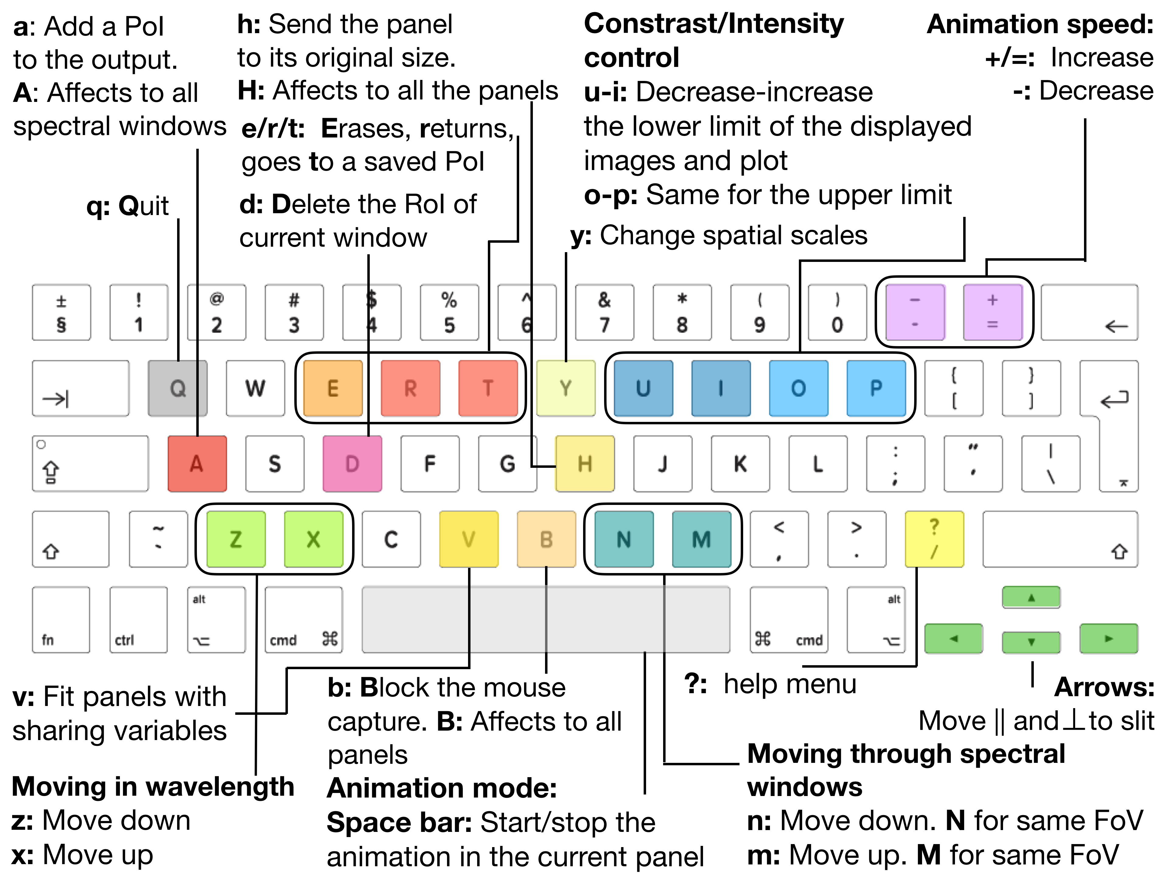
Fig. 3.6 The shortcut keys for ei.raster.quick_look and their meaning.

3.3. Customizing and initializing the visualization tool

Although the quick_look method allows to change many visualization parameters dynamically when the RoI or the SoI are being inspected, some basic ones can be directly changed from the attributes of these objects.

We can use the attributes from the RoI and SoI objects to make figures and plots manually and customize the aspect of the visualization.

Note

When show = True in iris_sji.build_figure or iris_raster.build_figure methods, the user can change the size of the figure by resizing the displayed matplotlib window. The new size will be automatically stored in the attribute figsize of window_label of the SoI or the RoI. This also happens when the visualization is done through the quick_look method. Thus, the user can play with the size of the IRIS SJI or raster viewer to get a figure more appealing in terms of aspect and white spaces between the panels.

If the user tries to adjust the spaces between panels with the “Adjust Tool” of matplotlib by clicking in the \(6^{th}\) icon shown in the Fig. 3.4, the “IRIS viewer” window losses the control of the keys. To recover the control of the keys the user can click in the “Save” icon (the \(7^{th}\) icon shown in the Fig. 3.4), and when the “Save” dialog window is open then press on the “Cancel” button.

The main attributes of the SoI, in our example of iris_sji.SJI['SJI_2796'] are:

• xlimN: the upper and lower limits of the X axis in the panel N, with N = 1 corresponding to the “SlitJawImage” panel, and N = 2 for the “SlideBar” panel.

• ylimN: the upper and lower limits of the Y axis in the panel N, with N = 1 corresponding to the “SlitJawImage” panel, and N = 2 for the “SlideBar” panel.

• clip_ima: the upper and lower limits of the values displayed in the “SlitJawImage” panel.

• cmap: the color map used to display the image in the “SlitJawImage” panel.

• slit_acqnum: the number of the slit-jaw image acquisition to be displayed.

• show_slit: if True, it plots a dashed line over the slit in the displayed slit-jaw image. Default is False.

• set_IRIS: if True, it sets the default values of a SoI, which include thresholds for the displayed images and plot, and the color map for the spectral window stored in the SoI.

Thus, we can customize or initialize the “IRIS SJI viewer”:

>>> iris_sji.SJI['SJI_2796'].xlim1 = [200, 700]
>>> iris_sji.SJI['SJI_2796'].xlim2 = [0, 30]
>>> iris_sji.SJI['SJI_2796'].clip_ima = [50,500]
>>> iris_sji.SJI['SJI_2796'].figsize = [5,6.5]
>>> iris_sji.SJI['SJI_2796'].slit_acqnum = 15
>>> iris_sji.SJI['SJI_2796'].show_slit = True
>>> iris_sji.quick_look()

or to make a figure and save it in a file with the keyword filename of the iris_sji.build_figure method (see Fig. 3.7):

>>> iris_sji.build_figure(show = True, filename = 'SJI_Mg_II_2796_seahorse_plage.pdf')

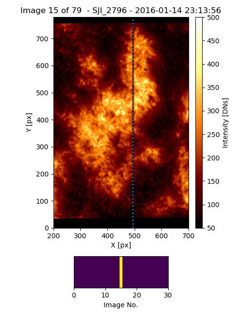
Fig. 3.7 Output of the customized iris_sji object.

We can also customize the iris_raster and create a PDF file of the resulting figure:

>>> iris_raster.raster['Mg II k 2796'].clip_ima = [50,500]
>>> iris_raster.raster['Mg II k 2796'].lim_yplot  = [0,900]
>>> iris_raster.raster['Mg II k 2796'].xlim1 = [50,100]
>>> iris_raster.raster['Mg II k 2796'].ylim1 = [40,110]
>>> iris_raster.raster['Mg II k 2796'].x_pos_ext = 66
>>> iris_raster.raster['Mg II k 2796'].y_pos_ext = 81
>>> iris_raster.raster['Mg II k 2796'].z_pos_ext = 2803.80
>>> iris_raster.raster['Mg II k 2796'].figsize =  [8.5, 7.21]
>>> iris_raster.raster['Mg II k 2796'].set_IRIS = False
>>> iris_raster.build_figure(window_label='Mg II k 2796', show=True,
>>>                          filename='example_build_figure.pdf')

or to initialize the quick_look:

>>> iris_raster.quick_look()

Thus, the visualization aspect is tighter, as we can see in Fig. 3.8:

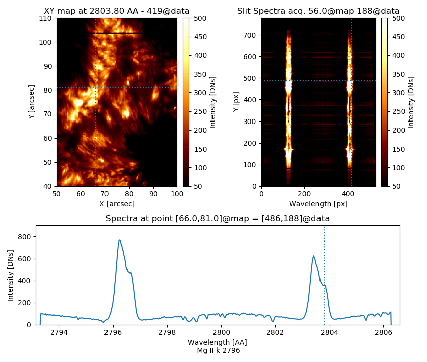
Fig. 3.8 Output of the customized iris_raster object.

Note that the method iris_raster.build_figure requires to have a valid loaded spectral window passed through the keyword window_label (“Mg II k 2796” in the example).

The main customizable attributes of iris_raster.raster['window_label'] are:

• xlimN: the upper and lower limits of the X axis in the panel N, with N = 1 corresponding to the “XY map” panel, N = 2 for the “Slit Spectra” panel, and N = 3 for the “Spectra” panel.

• ylimN: the upper and lower limits of the Y axis in the panel N, with N = 1 corresponding to the “XY map” panel, N = 2 for the “Slit Spectra” panel, and N = 3 for the “Spectra” panel.

• x_pos_ext: the position in the X axis in the “XY map” panel. It always given in the coordinates shown in that panel.

• y_pos_ext: the position in the Y axis in the “XY map” panel. It always given in the coordinates shown in that panel.

• z_pos_ext: the position in the Z axis of the “Spectra” panel. This value is given in Angstroms, since this panel is shown by default in these units.

• clip_ima: the upper and lower limits of the values displayed in the “XY map” and “Slit Spectra” panels.

• cmap: the color map used to display the images in the “XY map” and “Slit Spectra” panels.

• extent_display: the values of extent keyword, i.e the values of the X and Y axes in the “XY map” panel. The default available list of values accepted by this attribute is stored in output_variable.[window_label].list_extent.

• extent_display_coords: the coordinates corresponding to the extent_display. The default available list of values accepted by this attribute is stored in output_variable.[window_label].list_extent_coords.

• set_IRIS: if True, it sets the default values of a RoI, which include spectral positions of interest, thresholds for the images and plot displayed, and color map for each spectral window stored in the RoI.

Of course, we can use the RoI attributes to reproduce the “Spectra” of Fig. 3.8 using the standard plot utilities of matplotlib. Thus, we can do:

plt.figure(figsize=(12,3))
xdata = iris_raster.raster['Mg II k 2796'].wl
ydata = iris_raster.raster['Mg II k 2796'].data[486, 188,:]
ylim = iris_raster.raster['Mg II k 2796'].lim_yplot
plt.plot(xdata, ydata)
plt.ylim(*ylim)
plt.xlabel('Wavelength [AA]')
plt.ylabel('Intensity [DNs]')
plt.tight_layout()
plt.show()

In Section 2.6.2 we show how to make figures of the panels showed by the quick_look method from a PoI of a SoI or a RoI.