5. Observing with IRIS
5.1. IRIS day-to-day operations
Five times per week an IRIS planner makes a timeline that includes commands for pointing, observing sequences, downlinks, etc… for the next day (or several days). Planners start their timeline every weekday by 9 am PDT (Pacific Daylight Savings Time, i.e., 16 UTC). For example, the timeline that covers the time period from 4 UTC Tuesday until 4 UTC Wednesday must be completed by 16 UTC on Monday. The timeline is uploaded to the spacecraft and IRIS autonomously executes the commands. On Friday morning PDT the timeline for the weekend (which covers the time period from 4 UTC Saturday until 4 UTC Tuesday) is prepared. IRIS regularly conducts calibrations, in addition to a synoptic program of scientific observations. IRIS also performs extensive coordination with a variety of other observatories. The current IRIS coordination calendar can be found from the IRIS operations web-page.
5.2. IRIS data availability
IRIS data is automatically downlinked, typically within half a day of observing the Sun, followed by processing at the Joint Science Operations Center (JSOC) at Stanford and LMSAL. Typically quicklook slit-jaw movies are available online within 24 hours of recording the data onboard. The actual delay between observing and availability of quicklook movies depends on several variable factors, such as how full the onboard memory is. Quicklook data may not be perfectly calibrated (e.g., dark current or flat-field correction may not be perfect) because some of the calibration steps depend on instrument temperatures which require a few days to be processed and included. Final calibrated data is typically available within 7 days. IRIS has a public data policy, so data can be downloaded from the IRIS website. When using IRIS data in a publication, please use the following acknowledgement:
Note
When using IRIS data, please acknowledge IRIS as follows: IRIS is a NASA small explorer mission developed and operated by LMSAL with mission operations executed at NASA Ames Research center and major contributions to downlink communications funded by ESA and the Norwegian Space Centre.
5.3. IRIS eclipse season
IRIS is in eclipse season between the end of October and mid February of each year. This means that IRIS observations are interrupted during each orbit so that solar observations can only be performed for about 60 minutes out of every 97 minutes. Please note that no rolls are allowed during eclipse season.
5.4. How to request IRIS observations?
IRIS provides high-cadence, high-resolution imaging and spectroscopy of the chromosphere, transition region and select flare/coronal emissions. Furthermore, IRIS observations come with a variety of high-level data products, analysis tools, models, and experts to aid in analysis. IRIS is capable of flexible observing modes and rapid turnaround in targeting and delivering data on desired features.
If you are interested in obtaining IRIS observations (either in coordination with other observatories or from IRIS alone), please contact us at iris_request[at]lmsal[dot]com as soon as possible (ideally months in advance for coordinated observations, a week before for other types of observations) with your request.
Your request should include:
- science rationale
- target, desired roll angle
- requested day/time and duration
- key constraints and/or a suggested OBS-ID both for low-data rate (<0.5 Mbit/s) and high-data rate (~0.7 Mbit/s and higher) options, to take into account telemetry limitations.
- other participating instruments
- contact info
Once your observation request has been received and approved, it will be entered in the coordination calendar (if it is in coordination with other observatories). Two days before the observation, please contact the IRIS planner (who changes on a weekly basis but can always be reached at iris_planner at lmsal dot com) to confirm the approximate timing of your observation. Final targeting should be sent to the planner by 16 UTC on the day before the plan is to be uploaded unless the planner confirms otherwise.
For weekend timelines, the planner needs pointing for Saturday, Sunday and Monday by 16 UTC on Friday. For some holiday weekends 4-day timelines are uploaded, please check with your planner beforehand.
If you would also like to coordinate with Hinode, then please submit an IRIS-Hinode Operation Plan (IHOP).
- IHOPs are IRIS-Hinode Operation Plans
- Contact the Hinode team and IRIS PI (bdp at lmsal dot com) following the instructions on Hinode HOP page, including science justification, key constraints and requests for Hinode instruments and IRIS. For IRIS, this ideally is an initial guess for the OBS ID, duration and targets. These can be finalized after initial submission.
- IHOPs are discussed once per month for approval and observing during next month.
5.5. IRIS observing mode requirements and properties
To decide on the observing mode, it is best to look at previously obtained observations to understand what is involved in choosing IRIS observing programs (OBS). The full data archive can be accessed using IRIS Data Search Tool.
Please keep in mind that IRIS can, on average, download 0.7 Mbit/s (averaged over the whole day). While IRIS can support higher data rates for a limited time, it is best to keep data limitations in mind when formulating requirements. This can be done with the OBS Table Selector.
When formulating requirements for your desired IRIS observations, please go through the following list of choices:
5.5.1. IRIS wavelength choices
IRIS contains a slit-based imaging spectrograph that allows observations of:
- spectra in two wavelength ranges in the FUV (1331-1358 Å, 1390-1407 Å);
- spectra in a wavelength range in the NUV (2782-2834 Å);
- slit-jaw images (SJI) with bandpasses from a filter wheel that contains two bandpasses in the NUV (Mg II h/k 2796 Å and Mg II wing 2832 Å) and two bandpasses in the FUV (C II 1330 Å, Si IV 1400 Å).
At each timestep IRIS simultaneously takes FUV and NUV spectra as well as one of the four types of slit-jaw images. The slit-jaw bandpass can be different for each different timestep but only one slit-jaw bandpass can be taken at any one timestep.
For the FUV and NUV spectra, IRIS typically does not read out the full spectrum, but so-called linelists. This is done to reduce telemetry and means that only a subset of spectral lines are read-out and downlinked, depending on a given OBS.
5.5.2. Slit, spectral and spatial resolutions
IRIS has one slit, which is 1/3 arcsec wide. The imaging devices have 1/6 arcsec pixels with an effective spatial resolution of ~0.33 arcsec in the FUV and ~0.4 arcsec in the NUV. The slit can be moved across the solar disk with step sizes of 0.35, 1 or 2 arcsec up to a spatial range of roughly 120 x 175 \(\text{arcsec}^{2}\). The slit-jaw images cover a FOV of up to 175 x 175 \(\text{arcsec}^{2}\), while the slit has a length of 175 arcsec.
The spectral pixel size is 13 mÅ with an effective spectral resolution of ~27 mÅ in the FUV, and 26 mÅ pixels and effective spectral resolution of ~55 mÅ in the NUV. To boost signal-to-noise and/or reduce telemetry data can be summed onboard, both spectrally or spatially.
The highest spatial and spectral resolution (no onboard summing) is the default observing mode. Binning on the ground (i.e., after data was taken) can always be used during the data analysis stage, but summing onboard offers significant advantages:
- it lowers the data rate so observations can be run for a longer duration;
- it boosts the signal of faint lines above the digitization threshold (which on-the-ground summing cannot accomplish);
- it increases S/N so that exposure times can be lowered thus improving raster cadence.
Data can be summed onboard in the spatial direction (\(\times 2\), \(\times 4\)) or in the spectral direction (\(\times 2\), \(\times4\), \(\times8\)). A summing mode of \(1 \times 2\) would be no summing spatially, and \(\times2\) summing in the spectral direction.
Since the S/N in the NUV spectra is much better than in the FUV, there is also an FUV specific summing mode (\(\text{FUV} \times 2\), \(\text{FUV} \times 4\), \(\text{FUV} \times 8\)). Most used summing modes are probably \(\text{FUV} \times 2\) (spectral summing \(\times 2\) but only for the FUV spectra) and \(2 \times 2\) (i.e., spatial \(\times 2\), spectral \(\times 2\), for all channels).
Note
Asymmetric summing modes (e.g., \(1 \times 4\), \(2 \times 1\)) are typically discouraged since they lead to images with incorrect aspect ratio. If you desire asymmetric summing, please provide a detailed scientific rationale.
5.5.3. Cadence and exposure times
High throughput, fast readout and mechanism movements allow cadences for the spectra and slit-jaw images to be as short as 1.5-2 seconds. Available values for exposure times are 0.5, 1, 2, 4, 8, 15, 30 and 60 seconds.
Typical exposure times for bright lines such as C II 1335 Å, Si IV 1394/1402 Å are 2-4s and as low as 0.5-1s for Mg II h/k 2796 Å in active regions. For quiet Sun and coronal hole it is recommended to increase the exposure time up to 4-8s, and up to 15, 30 or 60s to detect fainter lines.
The exposure time is the same for FUV/NUV and SJI. It is typically a compromise value: it sets the signal-to-noise (S/N) of the observations, which depends on the type of target and also drives the raster (and SJI) cadence, as well as the data rate.
5.5.4. Signal-to-noise
The S/N consideration depends on the type of spectral lines observed. The S/N of the NUV spectra is much higher than for the FUV channel, so the FUV signal requirements usually set the exposure time. For the brightest lines in the FUV (C II 1335 Å and 1402 Å) reasonable signal can be obtained in:
- 2-4s for active regions
- 4-8s for quiet Sun and coronal hole
For fainter lines (e.g., O I 1355 Å, Fe XII 1349 Å), longer exposure times and/or summing will be required (as well as non-simultaneous readout and lossless compression).
Note
When pointing at active regions, the Automatic Exposure Control (AEC) algorithm usually operates to limit and reduce exposure times when large flares occur.
5.5.5. Duration, roll and pointing
An IRIS request needs to provide the time frame (in UTC) and the days for which support is requested. When choosing an OBS, please keep in mind that OBS with a high data rate may not be sustainable for a long time, depending on the other observing programs that are being run on the day of your observation. IRIS can sustain data rates of about 0.6 Mbit/s indefinitely, if IRIS is not rolled (roll angle = 0). If your desired OBS has a data rate that is above 1 Mbit/s, please provide an alternative, low data rate OBS (<0.5 Mbit/s) that can be used by the planner if the onboard memory is too full to run your high data rate version. Typically this would be a version with a longer exposure time, a summing mode, or a smaller line list.
The spacecraft can be pointed anywhere within 4 arcmin off the solar limb. IRIS can be rolled away from its usual solar south/north orientation by an angle between -90 and +90 degrees. A roll angle of -90 degrees means that the top part of the slit is oriented towards the East (i.e., slit rotated counterclockwise from solar north), while a roll angle of +90 degrees means that the top part of the slit is oriented towards the West (slit rotated clockwise from solar north). Note that we prefer roll angles of -90, -45, 0, 45, 90 (although others are possible too), and that we may not always be able to accommodate your roll angle, depending on the phase of the Moon (which would enter the field-of-view of our star tracker twice per month for a few days for certain roll angles), and during eclipse season (end of October through mid February every year). Non-zero roll angles can cause reduced telemetry (up to a factor of 2-3 lower in the worst case).
Note
For non-zero roll angles, the data rate that can be downlinked may be reduced by up to a factor of 2 because the X-band antenna is no longer pointing downward. In other words, requesting -90 degrees and 10 hours of a high data rate program may not be implementable.
For your initial request, please provide the type of target you want observations of so we can check whether the desired OBS is adequate for that type of target. Actual pointing information should be provided to the IRIS planner a day before the observations.
5.5.6. Field-of-view
IRIS has four different fields-of-view:
- very large (175” \(\times\) 175” for SJI, 175” along slit for spectra)
- large (120” \(\times\) 120” for SJI, 120” along slit for spectra)
- medium (60” \(\times\) 60” for SJI, 60” along slit for spectra)
- small (60” \(\times\) 60” for SJI, 30” along slit for spectra)
For coordinated observations with ground-based telescopes, medium is usually sufficient, unless the science goal aims to capture rare events like flares, CMEs, etc… in which case large or even very large may be preferred.
The required data rate scales with the field-of-view somewhere between linearly and quadratically.
5.5.7. Raster mode
IRIS can either operate in:
- sit-and-stare mode (slit stays at one location on the Sun)
- perform a raster scan.
The raster scan requires two choices to be made:
- step size: 0.35” (dense), 1” (sparse), or 2” (coarse)
- number of steps: 2, 4, 8, 16, 32, 48, 64, 96, 128, 192, 256, 320, 400.
The field-of-view of the sit-and-stare is 0.33” \(\times\) length of slit-read-out. The field-of-view of the raster scan (in the direction perpendicular to the slit) is then given by step-size \(\times\) number-of-steps, e.g., a dense 320 step raster scan covers about 105”. Note that not all combinations of dense/sparse/coarse with the number of steps are available.
5.5.8. Raster cadence
One you have decided on which type of raster you require, you should consider the raster cadence that results from your choice. This is given by:
- number-of-steps x (exposure time + overhead)
The overhead depends on how much of the detector you read out, but is typically of order 0.5-1.5 s. This means that a 320 step raster with 2s exposures can take up to 320 \(\times\) (2+1.5) = 1120 seconds, i.e., almost 20 minutes. Considerations for raster cadence:
- The larger the number of raster steps, the slower the repeat cadence.
- The cadence will be a compromise between how dynamic your events are, and what kind of spatial coverage you need to cover them adequately.
- Think of using a sparse or coarse step size to increase spatial coverage while reducing number of steps.
- To have a better raster cadence, consider reducing the exposure time and retaining signal-to-noise by summing onboard.
Exact raster timing can be obtained through the OBS Table Tool.
5.5.9. Slit-jaw type/cadence
There are four choices of slit-jaw filters:
- 2830, dominated by wing of Mg II h/k lines (photosphere), best for alignment with photospheric images from the ground
- 2796, dominated by Mg II k (chromosphere) and inner wings (photosphere), can be aligned with SDO 1600 and photospheric images from the ground
- 1330, dominated by FUV continuum (upper photosphere, low chromosphere) and C II 1335 Å lines (upper chromosphere, lower transition region), can be aligned with SDO 1600 (and some bright points are the same as photospheric/chromospheric images from the ground)
- 1400, dominated by FUV continuum (upper photosphere, low chromosphere) and Si IV 1394/1402 Å lines (transition region), can be aligned with SDO 1600 (and some bright points are the same as photospheric/chromospheric images from the ground)
For all desired observations, one should choose which slit-jaw filters should be used, with almost any combination of the 4 filters available. Keep in mind that these slit-jaw images cannot be taken simultaneously - one type of slit-jaw image is available per time-step (during which FUV and NUV spectra are always taken). So if all 4 slit-jaw types are desired, the fastest cadence of each individual SJI type is \(4 \times\) cadence of spectra.
It is possible to get any combination of 2796/1330/1400 at high cadence and combine it with a slower cadence for 2830 (for context).
Default observing modes are optimized to take each SJI as fast as possible. If the absolute highest cadence for each type is required, the request should indicate so. The fastest SJI cadence IRIS can provide would be a single channel (e.g., 2796) with short exposures of 2 s - the cadence would be of the order of 3 seconds in this case.
5.6. Linelists
While IRIS observes a spectral range from 1331-1358 Å, 1390-1406 Å and 2782-2834 Å, the full detector range is rarely read out and downlinked. This is to save telemetry and speed up the read-out. There are five pre-defined linelists to choose from. By default the medium line list is used. If a different linelist is desired, the request should indicate so.
The following five linelists have been predefined. The 80 million series is full readout and contains the full wavelength range in both FUV and NUV.
- Large Linelist
- Medium Linelist
- Small Linelist
- Flare Linelist
- Full Readout Linelist
The following figures illustrate the wavelength ranges covered by the linelists. Note that larger wavelength regions take longer to read out and affect the cadence. These also leads to larger downlink rates. The fastest cadence can be achieved with the small linelist.
5.6.1. Large Linelist
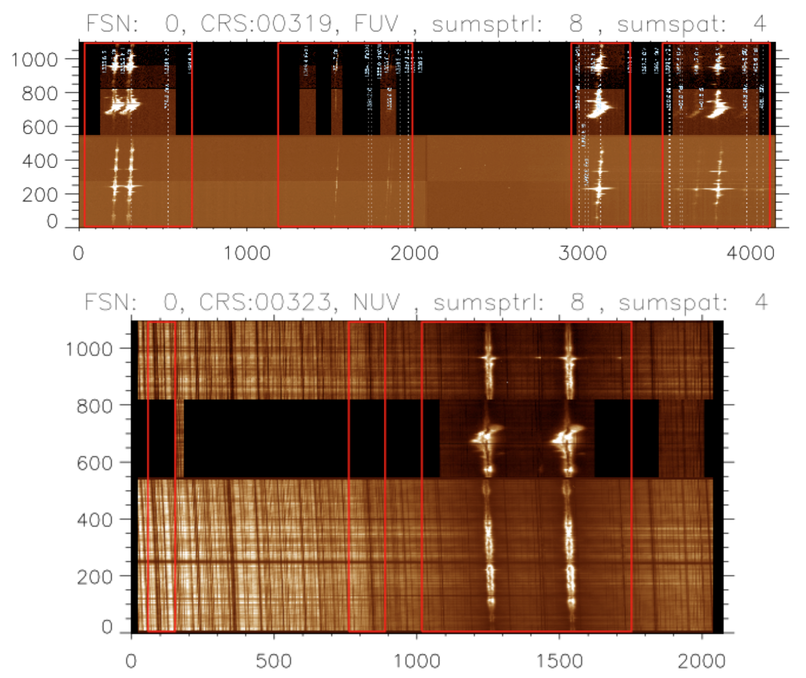
Large linelist. Regions of interest containing the selected lines are drawn as red boxes on real IRIS spectra.
FUV: Regions of interest containing the selected lines are downlinked.
NUV: A spectral region of about ~600 km/s (Doppler) around Mg II lines is read-out. Only linelist apart from flare and full read-out list that will also capture Mg II 3p-3d transitions for both lines.
5.6.2. Medium Linelist
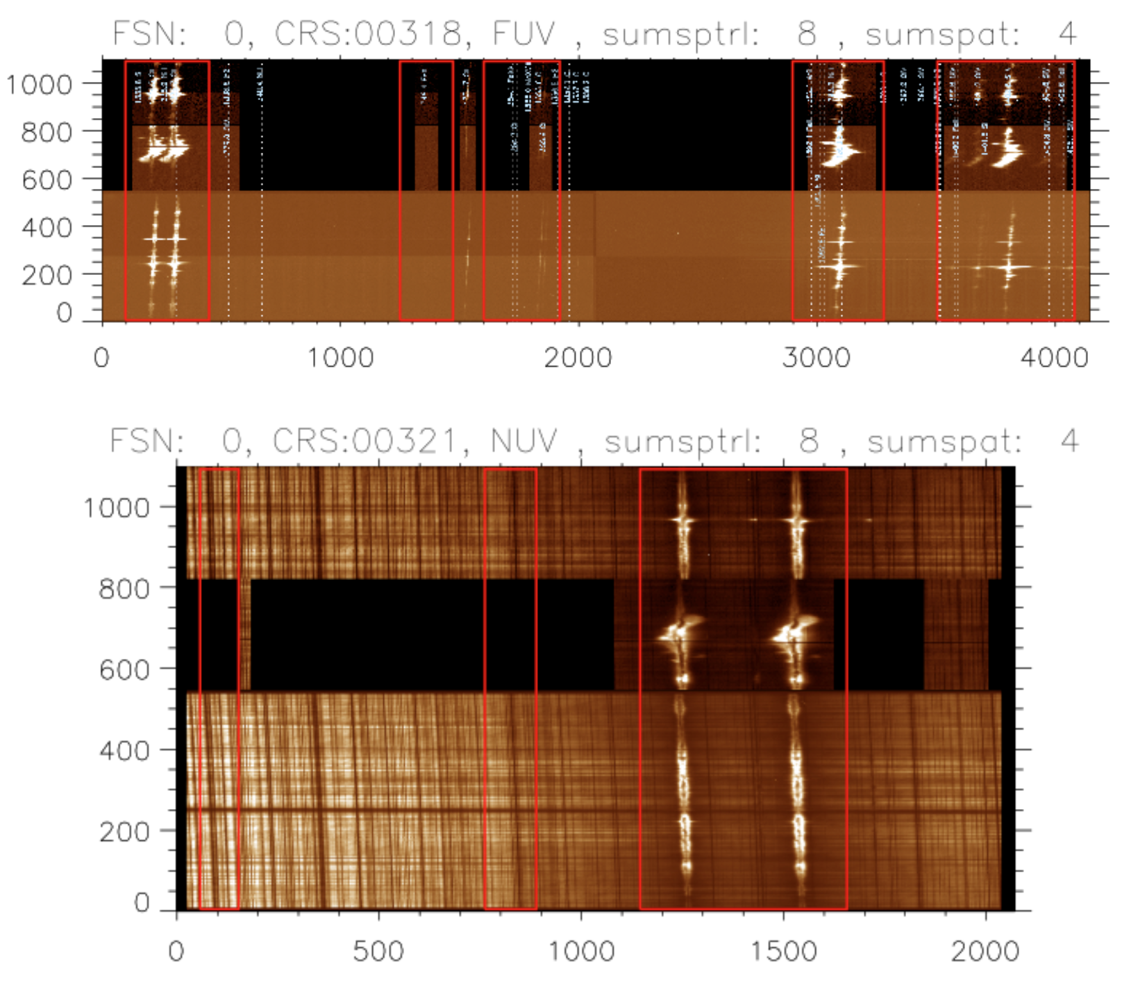
Medium linelist.
FUV: includes most lines, 300 km/s for most regions.
Medium: Both Mg II lines, photospheric reference line, plus continuum. ~300 km/s Doppler for Mg II.
5.6.3. Small Linelist
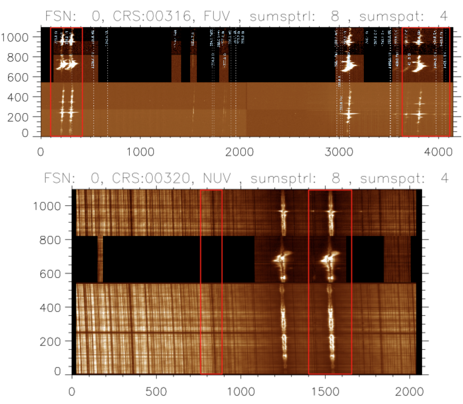
Small linelist.
FUV: minimal readout for fast observing programs, ~400 km/s Doppler shifts, focusing on Si IV and C II. No Fe XII or O IV 1399.
NUV: Only Mg II K line, plus photospheric reference. ~300 km/s Doppler.
5.6.4. Flare Linelist
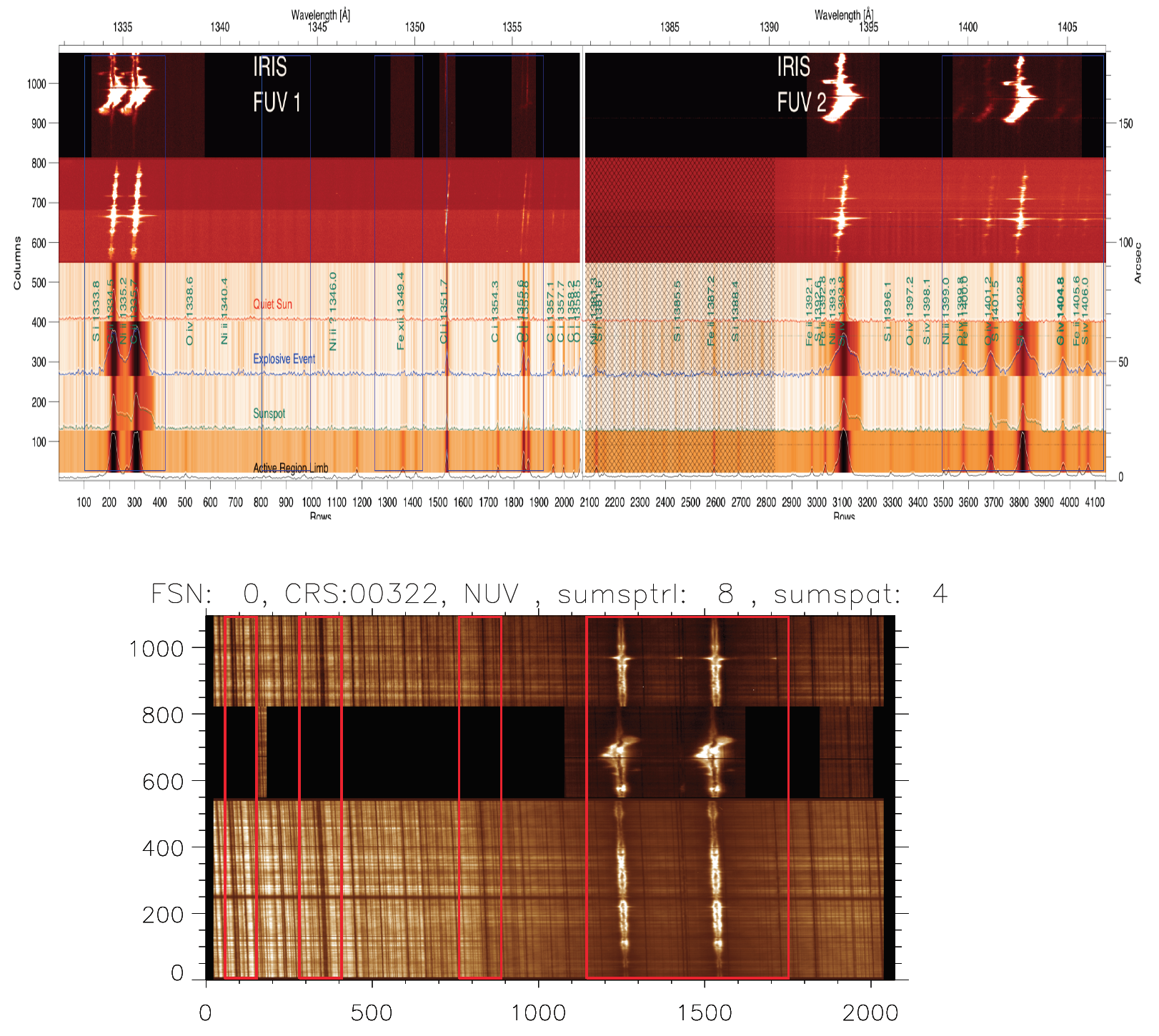
Flare linelist.
FUV: Si IV and CII. Both Fe lines (XXI and XII) and (allowed) O IV 1343.5 line (flare only). Also includes the S IV 1406 line to assist use of O IV 1399/1401/1404 density sensitive line pairs.
NUV: 600 km/s Doppler for blue wing.