6. IRIS planning tool

The selections made in section 5 can be easily translated to what the IRIS science planner needs to implement for an observational run using the OBS Table Selector. With this code, you can see the trade-offs between various OBS-ID possibilities, as explained below. IRIS has a range of different observing modes. The user can explore the observing parameter space with the table selector tool.

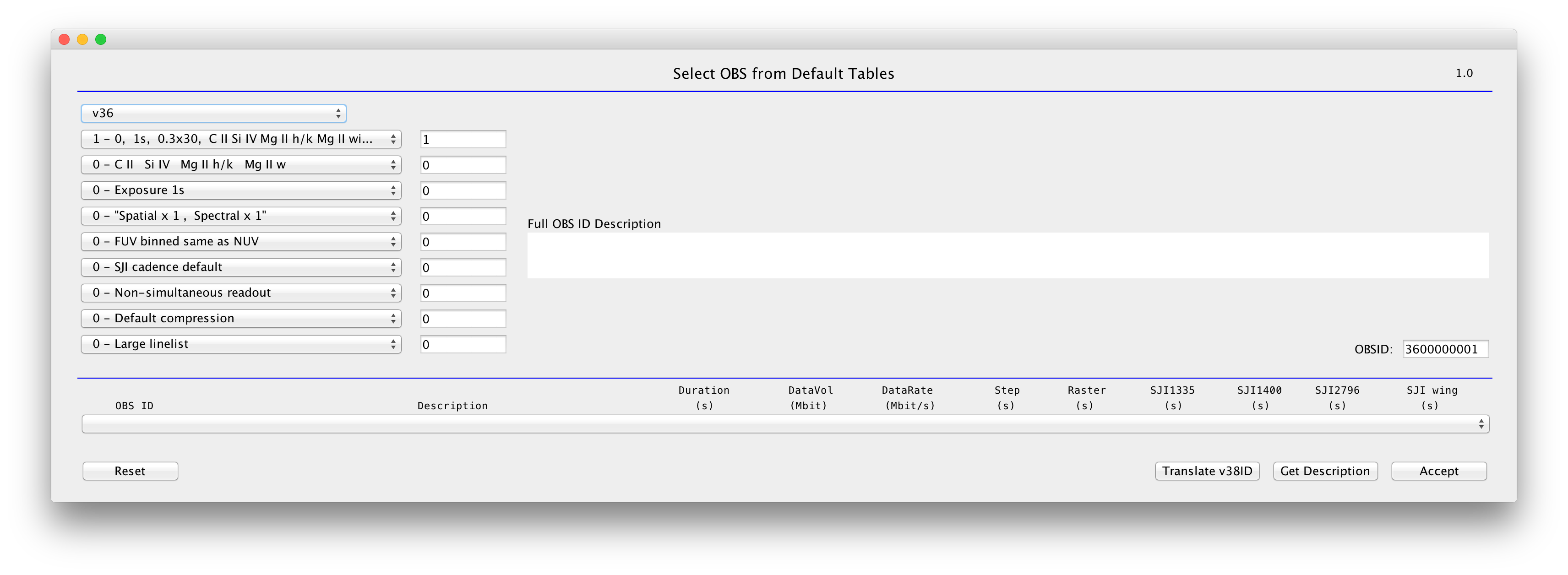
OBS-ID Table Selector.

For science observations, the IRIS science planner can choose from a variety of pre-defined or default observing tables. The identification number (OBS-ID) is a 16-bit integer whose value depends on the choices made in Section 5. The slit-jaw choices, cadence, raster type, exposure times are controlled by the OBS-ID numbers, as outlined in Table 3:

Table 3: OBS ID numbering scheme for table generation v3.6

OBS ID parent	Description
0-100	Basic raster type (sit-and-stare, rasters, …)
0-2,000	SJI choices
0-14,000	Exposure times
0-220,000	Summing modes (applied to FUV, NUV, SJI)
0-500,000	FUV summing modes
0-4,000,000	SJI cadence
0-5,000,000	Readout method (simultaneous, non-simultaneous)
0-10,000,000	Compression choices
0-80,000,000	Linelists
3.6-4 billion	OBS table generation number

Here are some details:

1. OBS-ID 0 to 1999: variations in cadence and wavelength choice of the four SJI filter images (C II 1335 Å, Si IV 1400 Å, Mg II h/k 2796 Å, Mg II h/k wing 2830 Å). Nominally cadence is ~10 seconds. If a “s” is following the wavelength, it means the cadence is slower (~60 seconds).
2. OBS-ID 2000 to 13999: variations in exposure time. Deep x 2 means exposure times are doubled, which lowers the cadence by roughly a factor of 2, etc.
3. OBS-ID 20,000 to 239,999: variations in onboard summing for the whole spectrograph (and imager).
4. OBS-ID 250,000 to 499,999: variations in onboard summing but applied only to the FUV spectra.
5. OBS-ID 1 million to 4 million: variations in SJI cadence.
6. OBS-ID 5 million: variations in read-out mode. Default (0) is non-simultaneous readout of the two science cameras. This is somewhat slower but avoids electronic readout noise (which affects FUV spectra the most) that is present during simultaneous readout (5,000,000). Unless extremely high cadence is critical, the default is preferred.
7. OBS-ID 10 million to 20 million: variations in compression.
8. OBS-ID 20 million to 100 million: variations in linelist (and thus cadence), including full readout.

There are three versions of the tables:

1. Version 3.6 is the most recent generation (as of May 2015) and contains optimized flare line list, and rasters. Requests should be made using version 3.6
2. Use of versions 3.8 and 4.0 is deprecated: these tables are only used if no equivalent is found in v3.6

To get an idea of the raster cadence, effective slit-jaw cadence and datarate, one can use the OBS Table Selector. This tool enables the use of the same drop-down menu that the IRIS planner uses when planning IRIS observations.

To investigate possible observing modes and compare the data rate (Mbit/s), raster cadence (sec) and slit-jaw cadence (sec) between various options, first either enter the OBS-ID in the field on the right (followed by ENTER and GET DESCRIPTION), or use the dropdown menu (followed by GET DESCRIPTION) as shown in the figure below. Ignore the “Duration” field, which is only for the IRIS planner’s benefit.

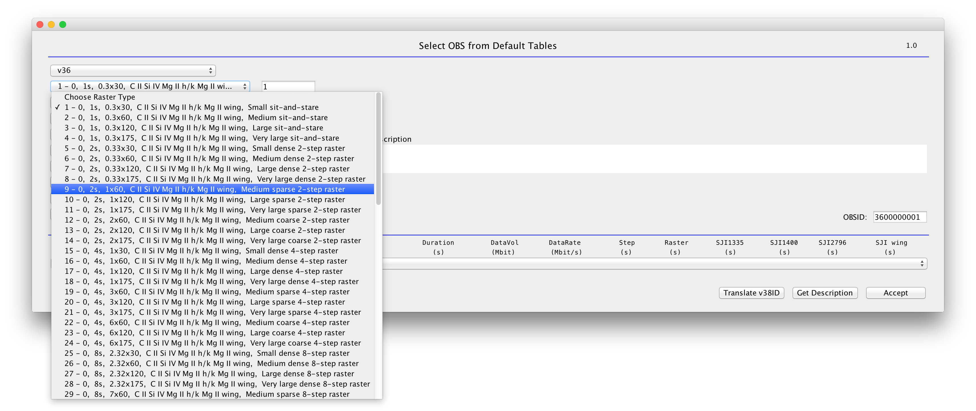
Dropdown menu for raster selection.

Once you have decided on which type of raster you require, you should select slit-jaw images type, their cadence and consider the raster exposure time that results from your choice.

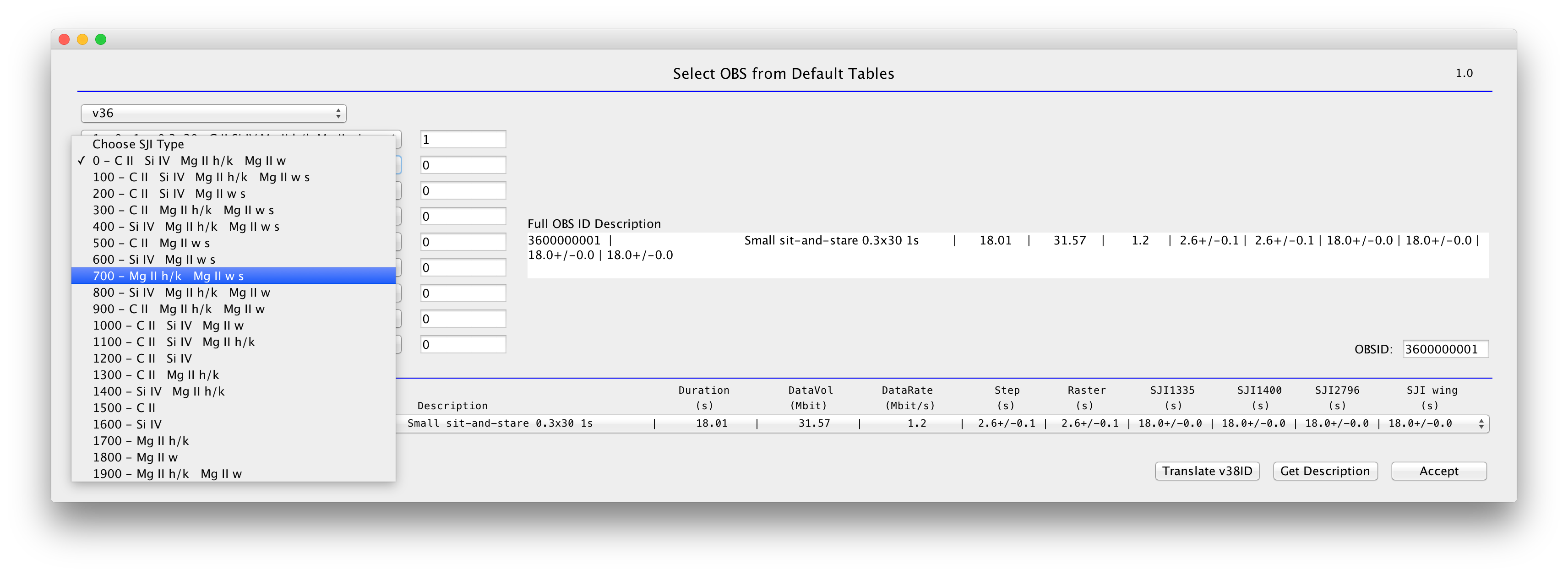
SJI types.

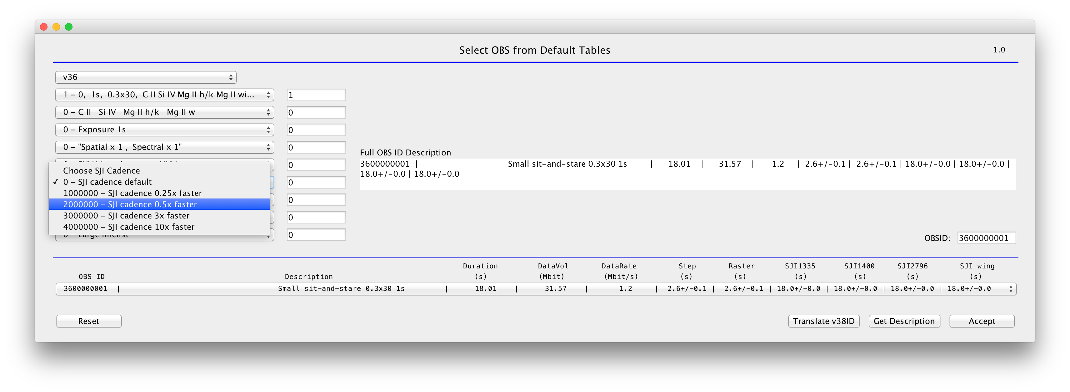
Possible adjustments of SJI cadences.

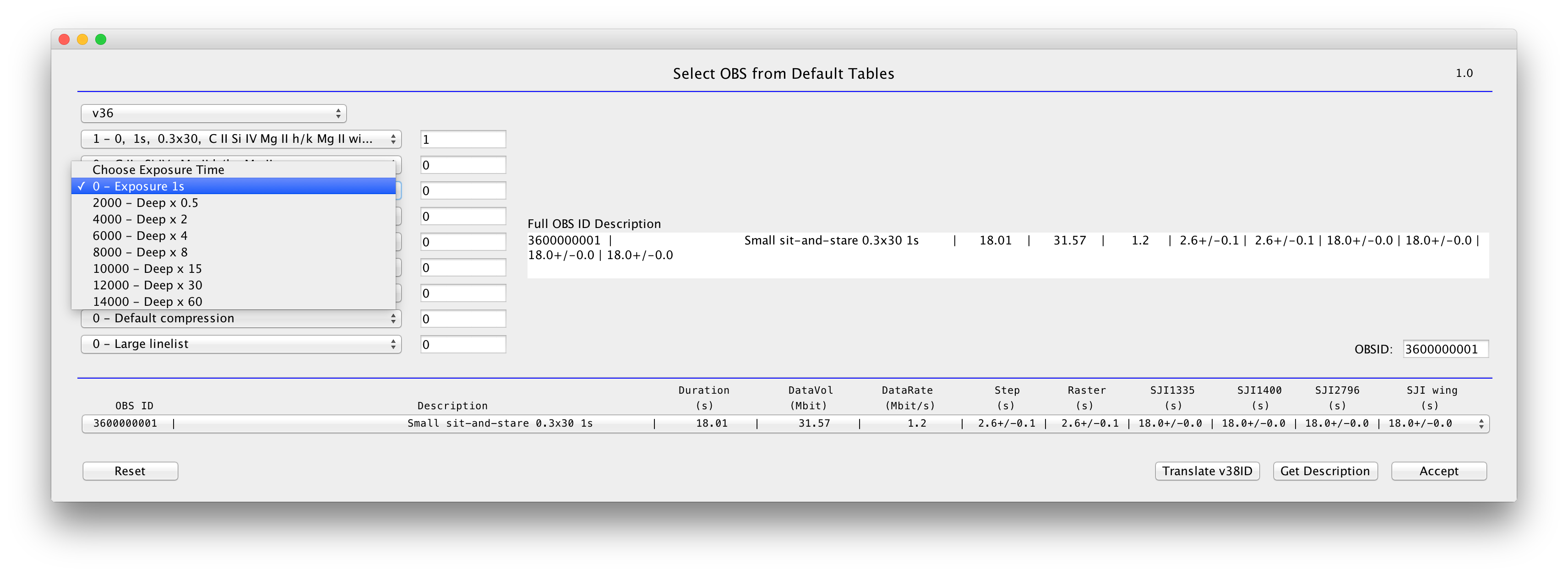
Exposure times.

Here we also have the option to adjust the highest spatial and spectral resolution. No onboard summing is the default observing mode. As previously mentioned, binning on the ground can be performed during the data analysis stage, but summing onboard provides some advantages:

• lower data rate ;
• stronger signal of faint lines;
• larger S/N.

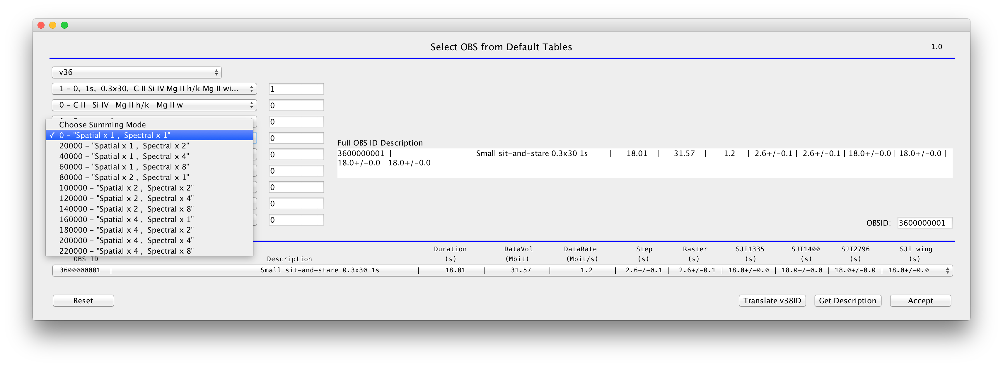
Spatial and spectral summing modes.

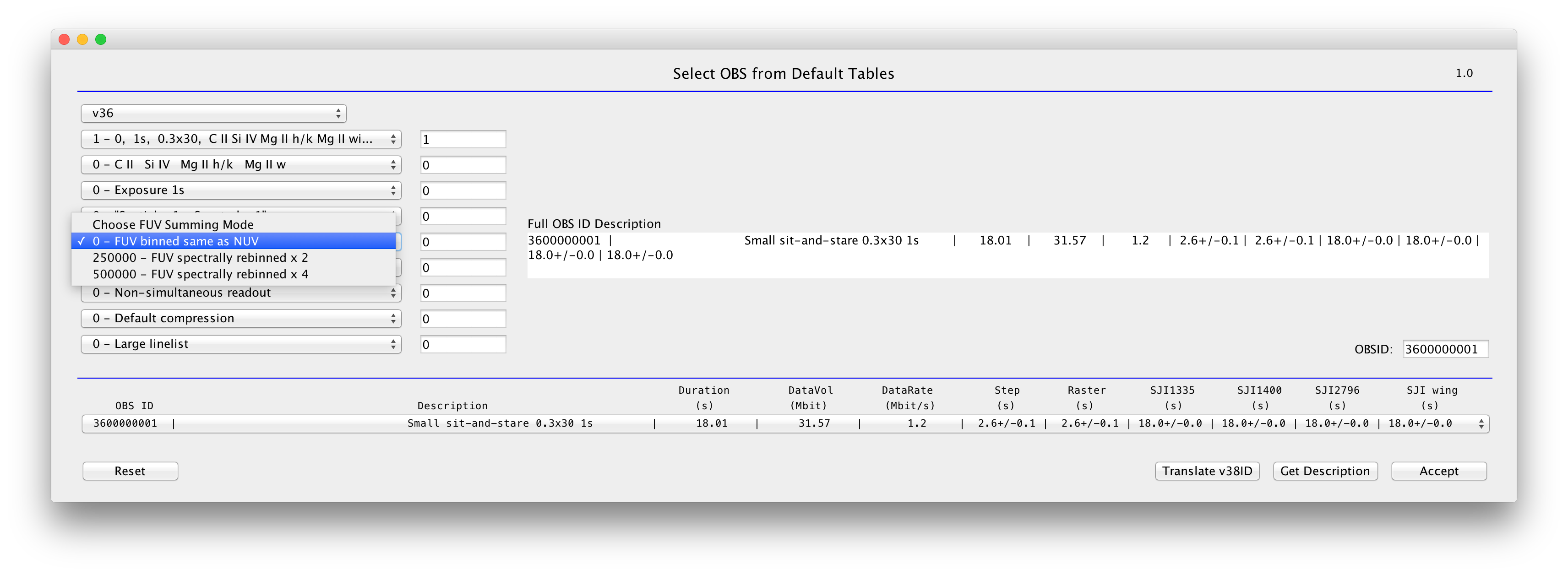
FUV spectral binning.

Non-simultaneous readout is default, which is adequate for most science goals. If very high cadence is critical, select simultaneous readout. Note that this leads to electronic read-out noise which can be very problematic for FUV spectra (given the lower signal-to-noise).

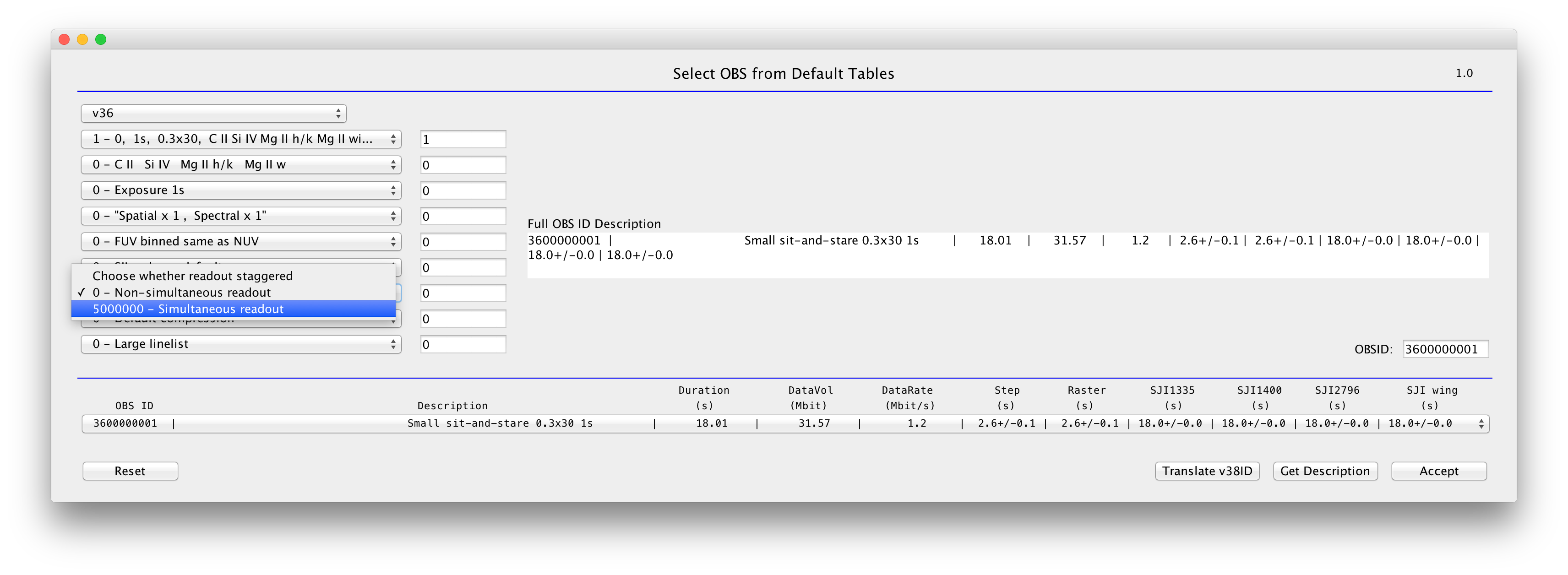
Readout options.

Lossy compression is default, which is adequate for bright lines and normal observations. If you are interested in faint lines, choose lossless compression. This leads to higher data rates.

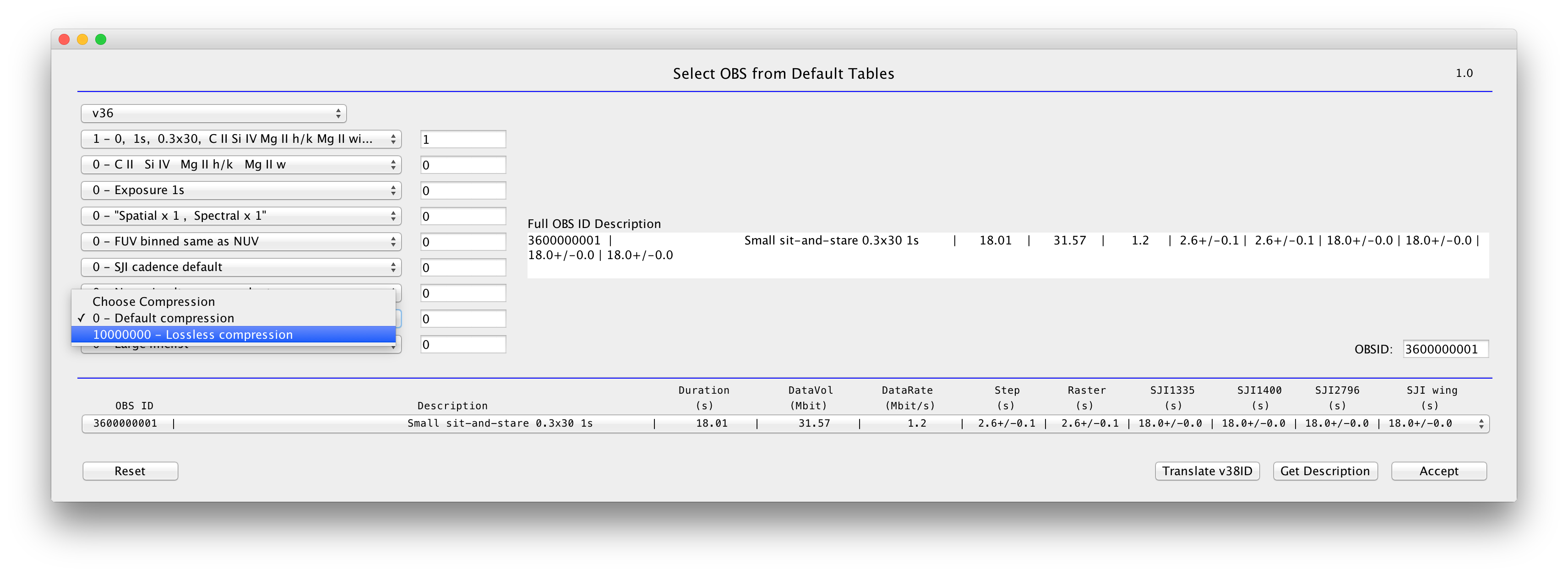
Compression selection options.

Other considerations:

1. Roll

Slit can be rolled up to +/- 90 degrees (e.g. to align with the limb, or cross the AR neutral line). Rolls can be limited on certain days (twice per month), or can impact telemetry rate. Work with the planner to determine optimal roll. The best option is to choose 0, +/-45 or +/-90 degree (for pointing stability).

2. Limb Observations

Generally it is best to have the slit on the disk for at least part of the observation. It is even better if the slit fiducial is on the disk. Consider rolling so the slit is parallel or perpendicular to the limb. Easiest co-alignment with ground based observations is through SJI 2832 (granulation), but also possible with 1400 or 2796.

3. Solar rotation tracking

Recommended for most observations, but can be left off for wide rasters, long runs, or limb observations.

4. SAA

Certain orbits are affected by particle storms (image spikes). If your observation is sensitive to these, request that the planner choose a time period to minimize SAA during your observation.

5. AEC

Automatic exposure control kicks in when there is a flare. Generally the planner will consider this (setting up the AEC if there is any chance of a flare in the field), but let them know if you think it should be disabled (e.g. you are looking for faint features in an active region).