4. IRIS Level 3 Data

IRIS Level 3 data permits the user to explore the connection between the slit-jaw imagers and the spectral data in one (time-)sequenced FITS file. The primary tool to navigate the Level 3 FITS files is called CRISPEX (the CRIsp SPectral EXplorer - developed for the CRISP instrument on the Swedish 1m Solar Telescope on La Palma by Gregal Vissers from the University of Oslo; http://folk.uio.no/gregal/crispex/). The current version is included in the IRIS IDL/SSW distribution so please take time to ensure that all of the Level 3 tools in your path are up to date. This can be done by updating the IRIS IDL SSW package.

4.1. Level 3 Data Structure

Level 3 data can exist in a variety of configurations. For a given observation, it combines multiple level 2 raster files into one or two level 3 files. The user can decide which spectral line windows to include in the level 3 file (e.g. include all the lines, only the NUV lines, or a selection), and so multiple level 3 files can be created from the same level 2 files.

There are two types of level 3 files: im and sp. They contain the same data, but one is the transpose of the other (this is to speed up access for visualization). The files are standard FITS files and the data is written in the primary Header Data Unit (HDU). The im files have the dimensions of (nx, ny, nwave, ntime), while the sp files have the dimensions of (nwave, ntime, nx, ny). Here ny is the number of pixels along the slit, and nx the number of steps in the raster; when rotation is used these are not aligned with solar (x, y) coordinates. For rasters with only one repeat (ntime = 1) the sp files are unnecessary and therefore not created. The different spectral windows of level 2 files are merged into the nwave dimension of the level 3 files.

Besides the primary HDU, level 3 files have three extensions, see below:

Ext. No.	Contents	Units	Dimensions
Primary	Main data	DN	(nx, ny, nwave, ntime)
1	Wavelength scale (vacuum units)	Å	(nwave)
2	Time of each exp. since DATE_OBS	Seconds	(nx, ntime)
3	Location of slit in SJI image	Pixels	(2, ntime, nx)

4.2. Creating Level 3 Data in IDL

IRIS Level 3 FITS files (documented in IRIS Technical Note 21) can be created in two ways (plus through two wrappers):

• Via iris_xfiles
• Via iris_make_fits_level3.pro - power user option. Can also be called through the wrapper iris_obsl223.pro - create level3 files for a given obs

Let’s look at an example of each.

Choose a raster file from iris_xfiles. You then get a window like this:

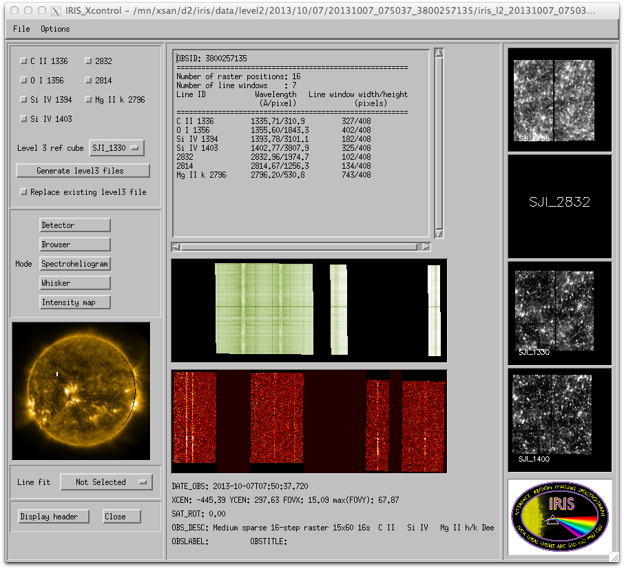
IRIS xfiles main interface.

In the upper left corner you can choose which lines to include in the level3 file and which SJI cube to use for reference. From the Options pull down menu you can choose the directory for the level3 files. Once the Generate level3 files button is selected, the progress is shown in the SSW terminal window where iris_xfiles was started. Using iris_make_fits_level3:

IDL> cd, getenv('IRIS_DATA') + '/level2/2013/10/07/20131007_054001_3800259115'
; where the environment variable IRIS_DATA should be the path to your IRIS data
IDL> f = iris_files('/*raster*.fits')
; the variable f is an array of raster files for that observation
; iris_files prints the file-names of all the raster files
; list the SJI files in the same folder
IDL> s = iris_files('*SJI*.fits')
; list the spectral windows possible, wdir is the directory where the level3
; files will be written, current directory is the default.
IDL> d=iris_obj(f[0]) & d->show_lines
0 C II 1336
1 O I 1356
2 Si IV 1394
3 Si IV 1403
4 2832
5 2814
6 Mg II k 2796
; we choose  C II, Si IV 1403, and Mg II k. You can choose all lines
; with keyword /all instead of the array with window indices
IDL> iris_make_fits_level3, f, [0, 3, 6], /sp, sjifile=s[0], $
        wdir=wdir, tmp_size=30

The second argument is the spectral window list that you want to study, in this example we’ve chosen [0, 3, 6], or C II, Si IV, Mg II h&k. The user should employ the tmp_size keyword, which sets the max temporary memory size, if a lot more memory than the default tmp_size of 12 GB is available. The unit is GB. The raster files go in the first argument, the desired spectral window(s) in the second - use the /all keyword instead of the second argument to get all windows, and the reference slit jaw image in sjifile (note that currently only one channel at a time is allowed). The /sp option produces a (lambda, time, x, y) cube in addition to the default (x, y, lambda, time) cube. This is only done if there is more than one raster file or if it is a sit-and-stare series. The routine will write the Level 3 data to directory wdir, default is the current working directory.

There is another optional argument to iris_make_fits_level3, called yshift. This can be used to correct for situations when the spectra and slit-jaws are not correctly aligned (e.g. issues with the automatic alignment). For more details on this calibration, see Coalignment between channels and SJI/spectra.

Looking in the working directory you now have:

IDL> f3=iris_files('*{im,sp}*fits')
0  iris_l3_20131007_054001_3800259115_t000_CII1336_SiIV1403_MgIIk2796_im.fits    1 GB
1  iris_l3_20131007_054001_3800259115_t000_CII1336_SiIV1403_MgIIk2796_sp.fits    1 GB

Note

These two Level 3 files are arranged differently but contain the same information. The im fits file is arranged by (X, Y, lambda, t) while the sp file, that is used by CRISPEX in the next section, is ordered (lambda, t, X, Y).

If one is working with many datasets, it may be advantageous to organize the level 3 files in a tree-structure similar to the level 2 files. This is easy to accomplish with the wrapper iris_obsl223. The example from above is then achieved with the call:

IDL> iris_obsl223, '20131007_054001_3800259115', iwin=[0, 3, 6], $
        /sp, rootl2=getenv('IRIS_DATA')+'/level2'

By default iris_obsl223 uses the 1400 SJI as reference slit-jaw cube. The level 3 root can be specified with the rootl3 keyword. The default is the same as rootl2 with the first string level2 replaced by level3. iris_obsl223 will create the directories necessary and will create symbolic links for the SJI images (with the iris_xfiles and iris_make_fits_level3 methods this has to be done manually).

4.3. Reading Level 3 Data in IDL

The level 3 files can be read in IDL with a regular FITS reader. For example, using readfits:

IDL> data = readfits('iris_l3_20140305_110951_3830113696_t000_all_im.fits', header)
% READFITS: Now reading 400 by 548 by 1410 by 1 array
IDL> help, data
DATA               FLOAT     = Array[400, 548, 1409]
IDL> wave = readfits('iris_l3_20140305_110951_3830113696_t000_all_im.fits', ext=1)
% READFITS: Reading FITS extension of type IMAGE
% READFITS: Now reading 1409 element vector
IDL> times = readfits('iris_l3_20140305_110951_3830113696_t000_all_im.fits', ext=2)
% READFITS: Reading FITS extension of type IMAGE
% READFITS: Now reading 400 element vector
IDL> help, times
TIMES           FLOAT     = Array[400]

In this example the level 3 file is from a single repeat raster, so the time dimension is collapsed when reading the data. Note that the main headers were read into the variable header. While one can also read the extension headers, most of the relevant information is in the main header.

4.4. Browsing Level 3 Data with crispex

4.4.1. Overview

crispex (http://folk.uio.no/gregal/crispex/) is called with an imcube, spcube (if there are more than one raster or a sit-and-stare series, it is always possible to call crispex with only imcube) and (optionally) a slit-jaw cube:

CRISPEX, imcube, spcube, sjicube=sjicube

If you are in the above example level 3 directory and have linked in the slit-jaw cubes (either manually or through running iris_obsl223):

; Exclude raster files if same directory contains any of those:
IDL> f=iris_files('*{im,sp,SJI}*fits')
IDL> f=iris_files()       ; enough if only level3 files in directory
0  iris_l2_20131007_054001_3800259115_SJI_1330_t000.fits      57 MB
1  iris_l2_20131007_054001_3800259115_SJI_1400_t000.fits      57 MB
2  iris_l2_20131007_054001_3800259115_SJI_2796_t000.fits      57 MB
3  iris_l3_20131007_054001_3800259115_t000_CII1336_SiIV1403_MgIIk2796_im.fits       1 GB
4  iris_l3_20131007_054001_3800259115_t000_CII1336_SiIV1403_MgIIk2796_sp.fits       1 GB
;It is then possible to start crispex using the f array
IDL> crispex, f[3], f[4], sji=f[1]

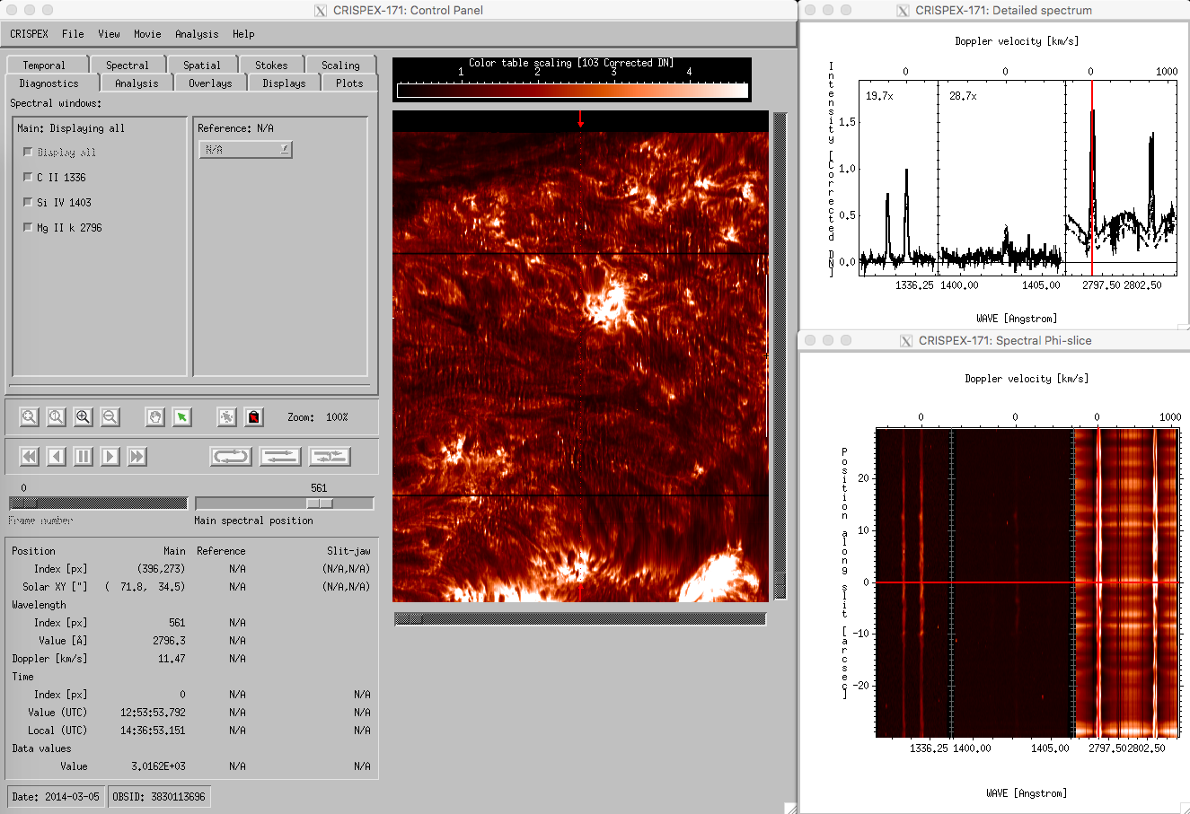
You will be greeted by a drop screen giving messages about the progress of the initialization. Then the crispex control panel, main detailed spectrum plot, spectral-T slice and the slit-jaw image will appear (window names written in blue here). The raster FOV for a given timestep and a given spectral position is shown in the control panel. This example dataset is a 4-step raster so it is very narrow and tall. There are eight tabs for the control of the behavior.

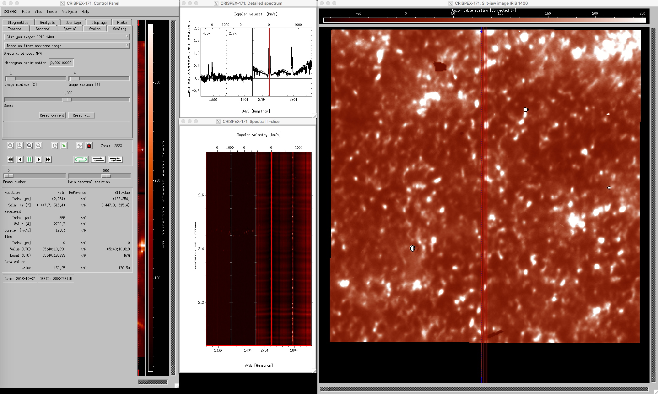
crispex main view with a 400-step IRIS raster.

The lower part in the control panel stays the same for all tabs. The timestep can be changed with the Frame number slider, the spectral position with the Main spectral position slider. Change the Main spectral position to 866 to get the spectroheliogram in the core of the MgII k-line. Note that a vertical line shows the spectral position in both the detailed spectrum window and in the Spectral T-slice window. When the Frame number is changed, a horizontal line in the Spectral T-slice window shows the position in time. When using the play buttons, the frame number is stepped through. When the cursor is moved around in the raster in the control panel, the Detailed spectrum window shows the spectrum at that position at the time given by Frame number. The Spectral T-slice window shows the temporal behavior of the spectrum at that position. It is possible to lock and unlock the position with the buttons in the control panel. The field below the lock and unlock buttons give values at the cursor position in different units.

crispex main view with a 4-step IRIS raster.

4.4.2. Tabs

The top part of the side panel is divided into several tabs. Here are short descriptions of their functions:

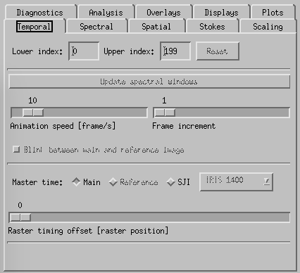
CRISPEX temporal tab.

Temporal-tab. The slit-jaw image is updated to be the closest in time to the time of the raster-step given with the slider Raster timing offset. It is possible to change the master time from Main (described so far) to SJI with the buttons above the Raster timing offset slider. In that case it is the slit-jaw frame number that is stepped by the play buttons and the raster closest in time to the slit-jaw is shown. To increase the speed of the movie in cases where there are many frames, one may change the speed with the Animation speed slider or increase the Frame increment with its slider. It is also possible to restrict the time-range with the boxes at the top of the temporal tab.

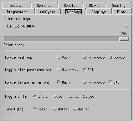
CRISPEX overlays tab.

Overlays-tab. The slit-jaw image has an overlay showing the position of the raster. This may be switched on and off (and color set etc) from the Overlays tab.

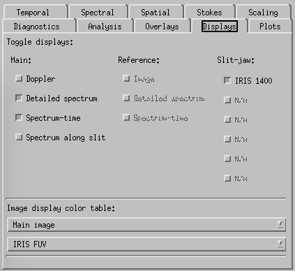
CRISPEX displays tab.

Displays-tab. Here one can switch on and off the various display windows and change the appearance of the Detailed spectrum plot. The lower and upper y-value can be set under the “Plots” tab. Switching on the Spectral-Phi display will show the spectrum along a slit shown in the raster in the control panel. The length of the slit and its orientation can be set in the spectral tab.

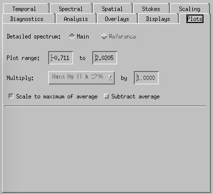
CRISPEX plots tab.

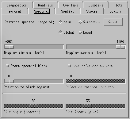
CRISPEX spectral tab.

Spectral-tab. Here it is possible to set the slit angle, slit length, slowly step the slit and set up a blink between two spectral positions (set the “Position to blink against” first and then the “Reference spectral position”. If there is only one line selected when producing the level3 file, it is possible to restrict the spectral indices in the top boxes.

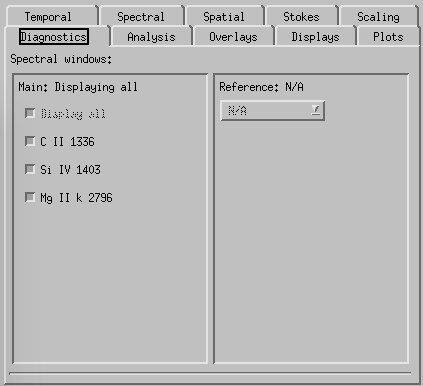
CRISPEX diagnostics tab.

Diagnostics-tab is used to select which of the lines to show in the various windows (default is all of them). Can also be used to control which detailed spectra of the available lines is shown on main window.

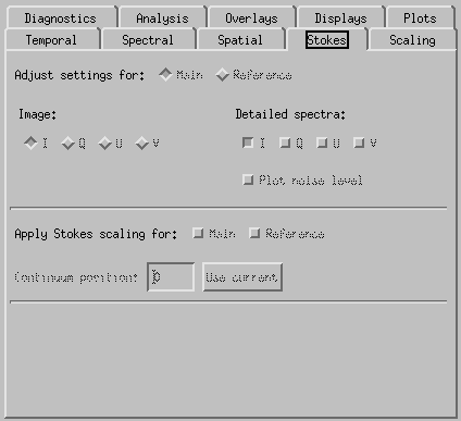
CRISPEX Stokes tab.

Under Stokes tab it is possible to select which element of the Stokes vector is show on main window. In case of IRIS, only intensity I is available.

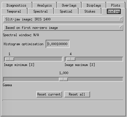
CRISPEX scaling tab.

Scaling-tab is used to set the scaling of all the image windows (min, max, gamma) and relative scaling of the various detailed spectrum plots. All line-windows are set separately so only the window where the main spectral position is is affected. The window to control is set in the top drop-down box.

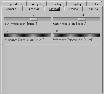
CRISPEX spatial tab.

Spatial-tab can be used instead of the cursor to set the (x,y) position within the raster.

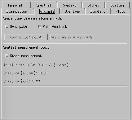
CRISPEX analysis tab.

Analysis-tab is used for some limited analysis like calculating space-time diagrams along a path. However, this has not yet been optimized for IRIS use.

This section will be expanded upon to provide the user more detail on:

• movie making,
• space-time plot construction,
• etc.

By far the best way to learn about crispex is by exploring, so try it. You can find detailed documentation for crispex at the IRIS documentation page and http://folk.uio.no/gregal/crispex/documentation.html