8. Useful codes

In this chapter we list a series of utility codes developed by the IRIS team that may serve as a basis for further investigations. The user is encouraged to use and study them, being aware of any assumptions and simplifications.

8.1. IRIS_getAIAdata

The routine iris_getaiadata is a graphical tool to download the AIA data that corresponds to a IRIS observation. The routine creates SJI-like level 2 files with the FOV fitted to the IRIS observation.

It is called in the following way:

IDL> iris_getaiadata, id

where id is a string that identifies a specific IRIS observation from the level 2 files. It can have three different forms:

• id = 'iris_l2_20131022_042024_3882010144_SJI_1330_t000.fits' (IRIS level 2 file)
• id = '/mn/xsan/d2/iris/data/level2/2014/02/01/20140201_090500_3880012095/ (directory name where a level 2 file exists)
• id = '20140410_051024_3882010194' (string with date and IRIS OBSID, for users that have a directory structure that mimics the IRIS data path, or a local data mirror)

Calling the routine will open a window with an overview of the parameters. One should choose an output directory where the AIA data will be saved, which AIA channels to save, and then confirm the values for XCEN/YCEN and FOVX/FOVY (a bug can sometimes result in them being incorrectly read). One can also extend the FOV and the time window. Finally, one can change the maximum number of files that will be downloaded per wavelength; the approximate temporal resolution is calculated whenever this number is changed. The highest cadence of AIA data is 12 sec, but this time interval can be larger.

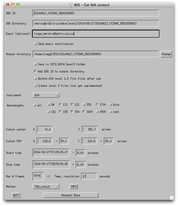
iris_getAIAdata dialog.

There are three options for downloading the AIA data:

1. SSW_cutout: This method downloads the AIA data via ssw_service, it first sends a request for a cutout of the data according to a IRIS OBS. This request is processed at LMSAL and can take from 5 min to a few hours. The download itself can also relatively slow. This method is recommended for large requests, when the full disk images will take long to download.
2. Full disk images: The full disk AIA data is first downloaded and then prepared locally. The files to download are very large, but the download speed can be higher when compared to ssw_cutout, and there is no waiting time for the data. This method is recommended for small and medium requests, for users with a good internet connection and plenty of disk space.
3. Archive: Does not download any data, assumes that the user has local access to /archive/sdo/AIA/lev1/. The preparation is done directly on the archived files. Max number frames is ignored, all available files are used. This mode is useful only for users at LMSAL.

After clicking on “Request Data” the window disappears, and the request is sent. Every few seconds the routine checks if the data are ready for download. At this point the tool can be interrupted, and restarted at a later time with:

IDL> IRIS_processAIArequest, outdir=outdir

The output of this routine will be one or more files similar in format to IRIS SJI level 2 FITS files, one file for each AIA channel. The header is the same as in the SJI FITS files, except that not all keywords are populated. The extensions of the FITS files are also in the same format as the SJI files, again, not all values are populated, because not all values are availabe in the AIA data. The data in the resulting fits files have the original AIA resolution, but are rotated to the same rotation as the IRIS data.

8.2. IRIS file handling routines

Several routines have been developed by Peter Young at NRL to handle IRIS files for users who don’t have a local mirror of the IRIS data. They are available in the IRIS Solarsoft directory (idl/nrl). See below for more details.

8.2.1. The $IRIS_DATA environment variable

This variable should point to where the user’s data files are stored, and it should be set in the .cshrc (or equivalent) or idl_startup.pro file. The variable can contain multiple paths. Example for idl_startup.pro file:

setenv, 'IRIS_DATA=$HOME/iris_data:/Volumes/DATA_DISK'

In this example the user has a data directory in his home directory, and another one on an external data disk. The software will search for files first in the home directory and then on the data disk.

8.2.2. Ingesting files

With $IRIS_DATA one can automatically transfer an IRIS file into the correct location within the IRIS directory tree using the routine iris_ingest.pro:

IDL> iris_ingest, local_file [, index=index]

By default the routine will put the file in the first directory path listed in $IRIS_DATA. To put it in another path, one can use the optional input index=. For example, index=1 will put it in the second path name (i.e., on the data disk in the example above). If you are not sure what the index numbers are, then do:

IDL> iris_ingest, /help

8.2.3. Finding files

With files correctly placed in the directory tree, one can find them from IDL using iris_find_file.pro. For example:

IDL> file = iris_find_file('29-Mar-2014 17:00')

By default this routine returns only the raster files, not the SJI files. To return the SJI files, use the keyword /sji. If the observation consists of multiple raster repeats, then the names of all of the individual files will be returned.

8.2.4. Finding a matching SJI file(s)

To find the SJI files corresponding to a given raster file, one can do:

IDL> sji_files = iris_sji_match(file)

8.3. IRIS dustbuster

The function iris_dustbuster cleans up the dust specs on the level 2 FUV SJI movies by picking good pixels from frames that are adjacent in time (so it works better on rasters, not sit-and-stares, though it’s safe to run on anything.

function iris_dustbuster, l2index, l2data, bpaddress, clean_values

Parameters:

• l2index – Index structure from a L2 SJI FITS file (read in using read_iris_l2)
• l2data – Data cube from a L2 SJI FITS file (read in using read_iris_l2)
• bpaddress – An N-element LONG array specifying the (1-D) address of the bad pixels in the L2 data cube
• clean_values – An N-element FLOAT array giving the pixel values to poke into the bad pixels

Returns: clean_data, A data cube with the same dimensions as l2data, with the dust busted (note that if the /list_only keyword is set, then only a scalar integer is returned (the user can do the replacement separately)

Usage:

cd, '/irisa/data/level2/2014/04/26/20140426_010036_3820257468/'
read_iris_l2, 'iris_l2_20140426_010036_3820257468_SJI_1400_t000.fits', l2index, l2data
cdata = IRIS_DUSTBUSTER(l2index, l2data, bpaddress, clean_values, /run)

8.4. IDL Routines for Level 2 Analysis

These codes are available in the IRIS SSW tree. They work with level 2 data.

pro iris_ne

Purpose: Derive the electron density from line pair intensity ratio and plot the result.

Required: The theoretical density-ratio files can be generated using CHIANTI:

density_ratios, 'o_4', 1398., 1402., 7., 13., den, rat, desc
d = interpol(alog10(den), 200, /spline)
r = interpol(rat,200,/spline)
save, filename='o4_1399to1401_den.sav', d, r

Usage:

int1 = [116., 56., 40.]    ; three intensities of O IV 1399Å
err1 = [17., 4., 5.]       ; the corresponding measurement error
int2 = [482., 155., 200.]  ; three intensities of O IV 1401Å
err2 = [25., 12., 10.]     ; the corresponding measurement error
den_file = 'o4_1399to1401_den.sav'
iris_ne, int1, err1, int2, err2, den_file, rat, rat_err, den, den1, den2

pro iris_ne_oiv

Purpose: Derive the electron density from the O IV 1401Å and 1399Å line pair.

Required: The theoretical density-ratio data is included in the code. So users do not need to retrieve this data from CHIANTI.

Usage:

int1 = [116., 56., 40.]    ; three intensities of O IV 1399Å
err1 = [17., 4., 5.]       ; the corresponding measurement error
int2 = [482., 155., 200.]  ; three intensities of O IV 1401Å
err2 = [25., 12., 10.]     ; the corresponding measurement error
iris_ne_oiv, int1, err1, int2, err2, rat, rat_err, den, den1, den2

pro iris_te

Purpose: Derive the electron temperature from line pair intensity ratio and plot the result. Joint observation between IRIS and EIS can be used to diagnose the electron temperature. Note that O IV 279.93Å/1401.16Å has little density sensitivity. Fe XII 195.12Å/1349.40Å has some density sensitivity but the density can be determined from EIS Fe XII line pairs.

Required: The theoretical density-ratio files can be generated using CHIANTI. For O IV:

temperature_ratios, 'o_4', 279, 1402, 4.5, 6.0, temp, rat, desc
t=interpol(alog10(temp), 250,/ spline)
r=interpol(rat, 250, /spline)
save, filename='o4_279to1401_temp.sav', t, r

For Fe XII (need to specify the density):

temperature_ratios, 'fe_12', 195, 1350, 5.5, 7.0, temp, rat, desc, density=10^8.5
t = interpol(alog10(temp), 250, /spline)
r = interpol(rat, 250, /spline)
save, filename='fe12_195to1349_temp_n8.5.sav', t, r

Usage:

int1 = [100., 200.]  ; two intensities of Fe XII 195Å
err1 = [12., 7.]     ; the corresponding measurement error
int2 = [1., 2.]      ; two intensities of Fe XII 1349Å
err2 = [0.05, 0.12]  ; the corresponding measurement error
temp_file = './NeTe/fe12_195to1349_temp_n8.5.sav'
iris_te, int1, err1, int2, err2, temp_file, rat, rat_err, temp, temp1, temp2

pro sgf_rbp_1lp, wvl, lp, ee

Parameters:

• wvl – wavelength vector
• lp – line profile
• ee – error vector

Purpose: Perform a single Gaussian fit to an optically thin emission line profile and derive an “RBp” profile as a function of velocity (this is a modified version of the “RB” line profile asymmetry analysis originally developed by De Pontieu et al. (2009, ApJ, 701, L1,) See the definition in Section 2 of Tian et al. (2011, ApJ, 738, 18,).

pro dgf_1lp, wvl, lp, ee, ini, range0, range1

Parameters:

• wvl – wavelength vector
• lp – line profile
• ee – error vector
• ini – initial guess
• range0 – allowed ranges of first component
• range1 – allowed ranges of second component

Purpose: Perform a double Gaussian fit to an optically thin emission line profile by supplying the initial guess of intensity ratio, 2nd component speed and width as well as the allowed ranges of the parameters for the two components.

Usage:

ini = [0.2, -50, 30]
range0 = [0.5, 2, 1]
range1 = [0.8, 2, 1]
dgf_1lp, wvl, lp, ee, ini, range0, range1

pro dgf_rb_1lp, wvl, lp, ee

Parameters:

• wvl – wavelength vector
• lp – line profile
• ee – error vector

Purpose: Perform RB and RBp-guided double Gaussian fit (see RBs in De Pontieu et al. 2009, ApJ, 701, L1,; see RBs, RBp, and RBd in Section 2 of Tian et al. 2011, ApJ, 738, 18,) for a single optically thin emission line profile.

function gen_rb_profile_err, v, profile, err, steps, dv

Parameters:

• v – vector of velocity from line centroid
• profile – line profile
• err – vector of measurement error at different spectral positions
• steps – velocity steps, e.g., [10, 20, 30, 40, …]
• dv – size of velocity bin, e.g., 20 km/s

Purpose: Get red wing and blue wing intensities of an optically thin emission profile as a function of velocity (spectral distance from line centroid). The result will be used to build an RB asymmetry profile.

pro tgf_1lp, wvl, lp, ee, ini, range0, range1, range2

Parameters:

• wvl – wavelength vector
• lp – line profile
• ee – error vector
• ini – initial guess
• range0 – allowed ranges of first component
• range1 – allowed ranges of second component
• range2 – allowed ranges of third component

Purpose: Do triple Gaussian fit to an optically thin emission line profile by supplying the initial guess of 2nd/core intensity ratio, 2nd component speed and width, 3rd/core intensity ratio, 3rd component speed and width, as well as the allowed ranges of the parameters for the 3 components.

Usage:

ini = [0.2, -50, 30, 0.05, 80, 20]
range0 = [0.5, 2, 1]
range1 = [0.8, 2, 1]
range2 = [0.8, 2, 1]
tgf_1lp, wvl, lp, ee, ini, range0, range1, range2

pro iris_nonthermalwidth

Purpose: Compute thermal and nonthermal widths in the unit of km/s.

Usage:

Wobs_v = 28.0        ; observed (1/e) line width in km/s
instr_fwhm = 0.026   ; instrumental FWHM in Å
Wnt_v = iris_nonthermalwidth('Si', 'IV', 1402.77, Wobs_v, instr_fwhm, ti_max=ti_max, Wt_v=Wt_v)

Notes: According to the IRIS paper, the spectral resolution (FWHM) is 26 mÅ in the FUV and 53 mÅ in the NUV.

pro iris_orbitvar_corr_l2, file, dw_orb_fuv, dw_orb_nuv, date_obs, (...)

Parameters:

• file – Level 2 file name
• dw_orb_fuv – the correction vector for orbital variation in FUV. Both the thermal and S/C velocity components are included. The unit is Ångström. (output)
• dw_orb_nuv – the correction vector for orbital variation in NUV. Both the thermal and S/C velocity components are included. The unit is Ångström. (output)
• date_obs – the vector of observation times
• dw_th – the thermal component of the orbital variation derived by using the Ni I 2799.474 (vacuum wavelength) line. The unit is unsummed wavelength pixel (about 0.0256 Ångström for NUV, 0.013 Ångström for FUV) (output)
• dw_sc – the spacecraft velocity (along the Sun-IRIS line) component of the orbital variation, positive value means the Sun is moving away from IRIS. The unit is km/s. (output)
• abswvl_nuv – the amount (unit Ångström) that has to be subtracted from the wavelengths if you want to do absolute wavelength calibration for NUV. (output)

Purpose: Purpose: Make corrections to the FUV/NUV spectral images for the spacecraft orbital variation of the spectral line positions using the Ni I 2799.474Å line for IRIS Level 2 FITS files. The input is a Level 2 spectrograph FITS file name. The iris_orbitvar_corr_l2s deals with a list of files.

Notes: dw_orb_fuv, dw_orb_nuv & date_obs saved into the file of datetime+'_orbitvar.genx', can be loaded using restgen, dw_orb_fuv, dw_orb_nuv, date_obs, file=datetime+'_orbitvar.genx'.

Note

The orbital variation (both the thermal component and the spacecraft velocity component) has been subtracted in the level 2 data generated from the May 2014 pipeline. The thermal component was evaluated using an empirical relationship between roll, temperature and line positions. In principle no further orbital variation correction is needed and the users can just use the level 2 data downloaded from the IRIS data website. The routine iris_orbitvar_corr_l2 can be used to correct for any data that has eventually not been properly calibrated.

pro iris_obs2hcr

Purpose: This function maps from IRIS OBSIDs, timelines and/or time range to create IRIS Heliophysics Coverage Registry (HCR) records http://www.lmsal.com/solarsoft/ssw/iris/idl/lmsal/util/iris_obs2hcr.pro (e.g., this is a wrapper for the general purpose ssw_hcr_query.pro suite of SSW codes). See the above URL for the doc-header for calling options and the ssw_hcr_query context example.

pro iris_obs2ssw_cutout

Purpose: A procedure to call the above - pulls IRIS-coordinated SDO images. Using IRIS HCR info, sets up and calls the SSW cutout service - http://www.lmsal.com/solarsoft/ssw/iris/idl/lmsal/util/iris_obs2ssw_cutout.pro

Usage:

IDL> iris_obs2ssw_cutout, '20140610_072252_3820011653', fov_expand=60, $
        minute_window=5, blend_waves='304,193,171', $
        description='IRIS_Vortex_SST', max_frames=500, $
        max_movie_frames=500, email='your@email.here’

This calls iris_obs2hcr.pro to get IRIS time/pointing specifics, then calls the aia/sdo ssw cutout service (ssw_cutout_service.pro) using those windows, optionally expanded (+/-60” & +/- 5 minutes in above example) - cutout service inherits any keywords (max_frames, blend_waves, etc) as described in http://www.lmsal.com/solarsoft/ssw_servic/ssw_service_track_fov_api.html

Output of the above:

Job Summary (service parameters per call, job/size summary)
http://www.lmsal.com/solarsoft/ssw_service/queue/finished/ssw_service_140618_113133_38871.html

-> WWW/movie summary (via link in above summary)
http://sdowww.lmsal.com/sdomedia/ssw/media/ssw/ssw_client/data/ssw_service_140618_113133_38871/www/

Retrieve the AIA/HMI FITS cutout data from above -> local (see get data cut & paste line in Job Summary) - optionally, specify output directory and WAVES list (default=Current and All, resp.) - here I ask for SDO/AIA 193Å and SDO/HMI Blos only - cut & paste this into IDL session:

(...)
IDL> ssw_service_get_data, "ssw_service_140618_113133_38871", /loud, waves='193,blos'