1. Introduction
1.1. About this Guide
This guide is written as a “cookbook” to help novice IRIS users through the steps of how to acquire data, reduce it, and perform some data analysis. It provides an overview of the instrumental capabilities, how the data is organised and calibrated, and how to read and interact with it.
If you are in a hurry or pressed for time, we suggest you go straight to Quickstart. You can then go through the other chapters to get more detail of a particular topic.
This introductory chapter provides an overview of the instrument, data products, operations, and where to find technical documentation. After familiarising themselves with the instrument, we encourage all new users of IRIS data to start with the Level 2 chapter.
This guide is evolving and is frequently updated. It is a collaborative effort and is currently maintained by Tiago Pereira. Much of this guide comes from the tireless work of Scott McIntosh, who steered the guide from the early days of IRIS when the tools and data calibration were changing quickly. Please email astro.uio.no@tiago.pereira (reverse user/domain) with corrections or questions, and we will respond as soon as possible.
This cookbook is a guide for browsing IRIS data before further analysis - a “quicklook” guide. The codes/tools discussed for data analysis will be black boxes to the non-expert user, but those codes are simple in structure and we encourage the user to study them and use them to analyze the IRIS data that they have downloaded. Please keep in mind that there are always assumptions and simplifications made in applying a priori physics to line spectra analysis, e.g., is an optically thin emission line profile best represented by a Gaussian?
1.2. IRIS instrumentation
IRIS is the Interface Region Imaging Spectrograph small explorer (NASA Small Explorer- SMEX). The IRIS investigation combines advanced numerical modeling with a high resolution, high throughput multi-channel UV imaging spectrograph fed by a 20 cm UV telescope. The main science goal of IRIS is to understand how the solar atmosphere is energized. IRIS obtains UV spectra and images in two main passbands around 1400Å and 2800Å at high resolution in space (0.33-0.4”), time (1s) and spectrally (~26 and ~53 mÅ respectively) that are focused on the chromosphere and transition region including some coverage in the corona.
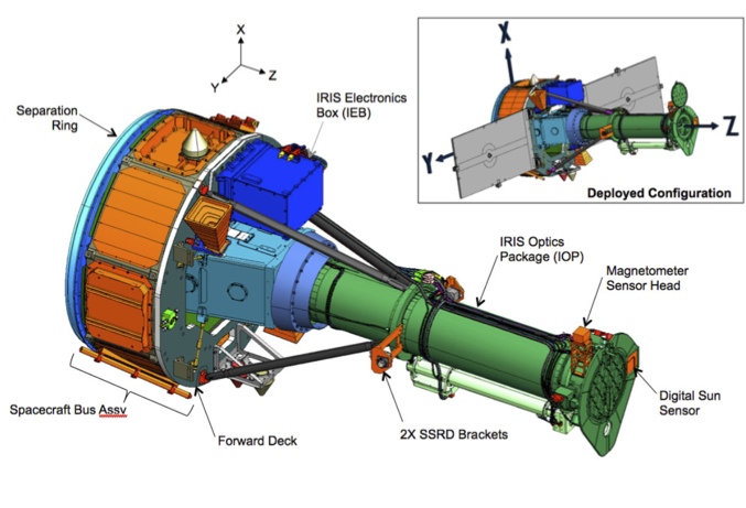
Schematic view of IRIS showing the 20 cm UV telescope, with and without solar panels (for clarity). Light from the Cassegrain telescope (green) is fed into the spectrograph box (light blue).
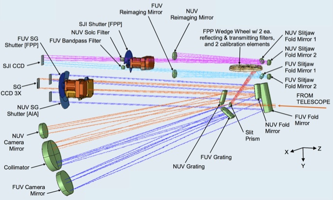
Schematic diagram of path taken by light in the FUV spectrograph (dark blue), NUV spectrograph (orange), FUV slit-jaw (light blue) and NUV slit-jaw (purple) path.
The IRIS telescope feeds light from three passbands into the spectrograph box:
- Far Ultraviolet (FUV1): 1331.56–1358.40 Å
- Far Ultraviolet (FUV2): 1390.00–1406.79 Å
- Near Ultraviolet (NUV): 2782.56–2833.89 Å
In the spectrograph, the light follows several paths (see spectrograph schematic), either:
- Spectrograph (SG): passing through a slit that is 0.33 arcsec wide and 175 arcsec long, onto a grating that is sensitive in both FUV and NUV passbands, then onto 3 CCDs to produce spectra in three passbands (FUV1, FUV2, NUV; Table 1)
- Slit-Jaw Imager (SJI): reflected off the reflective area around the slit (“slit-jaw”), passing through or reflected off broadband filters on a filterwheel, then onto 1 CCD to produce an image of the scene around the slit (slit-jaw = SJI) in 6 different filters (2 for calibration, 4 for solar images, Table 2)
Exposure times are controlled by 3 different shutters (FUV, NUV and SJI). Light is collected onto 4 CCDs which are read out by 2 cameras (see Section 3 for details) and which cover 3 different spectral bands and the slit-jaw images (Table 1, 2). The IRIS spectral lines cover temperatures from 4,500 K to 10 MK, with the images covering temperatures from 4,500 K to 65,000 K (and possibly 10 MK under flaring conditions). See IRIS Technical Note 1 for more details on IRIS.
Table 1. Overview of spectrograph (SG) channels. These are imaged onto 3 identical 1096x2072 pixel2 CCDs and can all be simultaneously read using two different camera electronics boards (CEB). Ranges, dispersion and effective area are current best estimates based on pre-launch measurements. Spatial pixel size is 0.166”, and the maximum spatial extent is 175”.
| Band | Wavelength (Å) | Dispersion (mÅ/pix) | Effective area (cm2) | Temperature (log T) |
|---|---|---|---|---|
| FUV 1 | 1331.7–1358.4 | 12.98 | 1.6 | 3.7–7.0 |
| FUV 2 | 1389.0–1407.0 | 12.72 | 2.2 | 3.7–5.2 |
| NUV | 2782.7–2851.1 | 25.46 | 0.2 | 3.7–4.2 |
Table 2. Overview of slit-jaw (SJI) channels. Slit-jaw passbands are chosen using a filterwheel. The light is imaged onto one 2072x1096 pixel CCD with only one passband exposed/read-out at one time. Read-out is done with the same CEB as NUV SG. Ranges, full width half max (FWHM), and effective areas of the passbands are best estimates based on pre-launch measurements. SJI passband types are either mirrors (M) or transmission filter (T). Spatial pixel size is 0.166”, and the spatial range is 175”x175”.
| SJI Passband | Type | Wavelength (Å) | FWHM (Å) | Effective area (cm2) | log T |
|---|---|---|---|---|---|
| Glass | T | 5000 | 2000 | – | – |
| C II | M | 1330 | 40 | 0.5 | 3.7–7.0 |
| Si IV | M | 1400 | 40 | 0.6 | 3.7–5.2 |
| Mg II h/k | T | 2796 | 4 | 0.005 | 3.7–4.2 |
| Mg II wing | T | 2832 | 4 | 0.004 | 3.7–3.8 |
| Broad-band | M | 1600 | 400 | – | – |
Table 3. IRIS data level descriptions.
| Level | Processing | Notes |
|---|---|---|
| TLM | Capture
|
Raw telemetry
|
| 0 | Depacketized
|
Raw images with basic keywords
|
| 1 | Reorient images to common axes:
North up (0° roll),
increasing wavelength to right
|
Lowest distributed level
|
| 1.5 | Dark current and offsets removed
Flag bad pixels and spikes pixels
Flat-field correction
Geometric and wavelength calibration
|
Transitory data product for level 2
production. Not distributed,
for internal use only.
|
| 1.6 | Physical units (exposure and photon
conversion)
|
Not distributed.
|
| 2 | Recast as rasters and SJI time series
|
Standard science product.
Scaled and stored as 16-bit images
|
| 3 | Recast as 4D cubes for NUV/FUV spectra
|
CRISPEX format |
| HCR | Description of observing sequences
|
Ingested by HCR at LMSAL.
To be searched by VSO, etc.
|
1.3. IRIS Data Level Definitions
The convention on IRIS Data Levels is shown in the table above and at length in IRIS Technical Note 11. Raw spacecraft telemetry is converted into Level 0 image files. Level 1 images are reoriented so that wavelength increases left to right.This constitutes the lowest level of scientifically-useful data, however since it is uncalibrated, Level 2 is the correct data product for most analyses. However, if an end user desires to download level 1 data (despite the fact that it is NOT recommended!), it can be done using the following IDL commands (more details about IRIS SolarSoft package is provided in Section 1.5 and Section 2):
;for example for observations taken from '18:50:00 10-nov-2014' until '19:00:00 10-nov-2014'
IDL> t0 = '18:50:00 10-nov-2014'
IDL> t1 = '19:00:00 10-nov-2014'
IDL> urls = iris_time2files(t0, t1, level=1, /urls)
IDL> sock_copy, urls
The type of processing for data Levels beyond 1 is dependent on whether the data is from the slit-jaw imager or spectrographs. Darks and pedestal offsets are removed, and flat-fielding corrections for telescope and CCD properties are applied to generate Level 1.5 data. The data at Level 1.5 has had the geometric and wavelength corrections applied and the images are mapped to a common spatial plate scale. Spectral images are remapped to align with an equal-sized array where wavelength and spatial coordinates align with the grid. An array mapping the wavelength axis to physical wavelength is created in this process. As with AIA, equivalent procedures to those used internally to transform level 1 to level 1.5 are distributed via SolarSoft as iris_prep.pro [http://sohowww.nascom.nasa.gov/solarsoft/iris/idl/lmsal/calibration/iris_prep.pro].
Levels 2 and 3 are generated from Level 1 or Level 1.5 data and are reorganized so that they can be analyzed using tools adapted from Hinode/EIS and SST/CRISP. Level 2 data consists of sets of 3D image extensions of each wavelength band stored as (λ,x,y) assembled from rasters of NUV and FUV Level 1.5 data. Level 3 data exist only for spectral rasters, and are 4D datacubes stored as (x,y,λ,t). We will describe some of those tools below.
Note
Level 1 vs. level 2 data: This guide is written with the general solar physics community in mind. In the following sections we will discuss IRIS data retrieval and analysis. The spectral data of IRIS is distinct from many contemporary observatories like SDO. IRIS Level 2 data is equivalent to Level 1 data products of those other observatories. The Level 2 data are fully reduced, calibrated, etc. and packaged such that they are “shovel ready” for further analysis. On the other hand IRIS Level 1 data MUST be passed through the calibration routines iris_prep.pro by the expert user to reach only level 1.5. The transition from level 1.5 to level 2 is a non-trivial exercise in packaging the data and while the code is available, it is currently not being supported for general use. Therefore, we strongly recommend that the non-expert or casual IRIS user use the Level 2 data products.
1.4. Sample IRIS data
1.4.1. Sample Spectra and the NUV/FUV Lines
These sample spectra taken by IRIS show the number of counts per pixel per second in a 15 second exposure in several solar regions (plage, sunspot, and network). You can see the strong lines in each spectral range and their relative strength in regions with different degrees of activity. Using the very narrow photospheric lines in each channel we estimated that the spectral resolution (2 x the Nyquist sampling of the spectrograph) of the FUV spectra is 25mÅ and 60mÅ for the NUV. Indeed, those narrow photospheric lines, because they typically display very small intrinsic velocities and broadening (~1km/s in each), are used for wavelength calibration and the geometric correction steps in the spectrographic data. IRIS Technical Note 20 and IRIS Technical Note 19 cover these processes in detail.
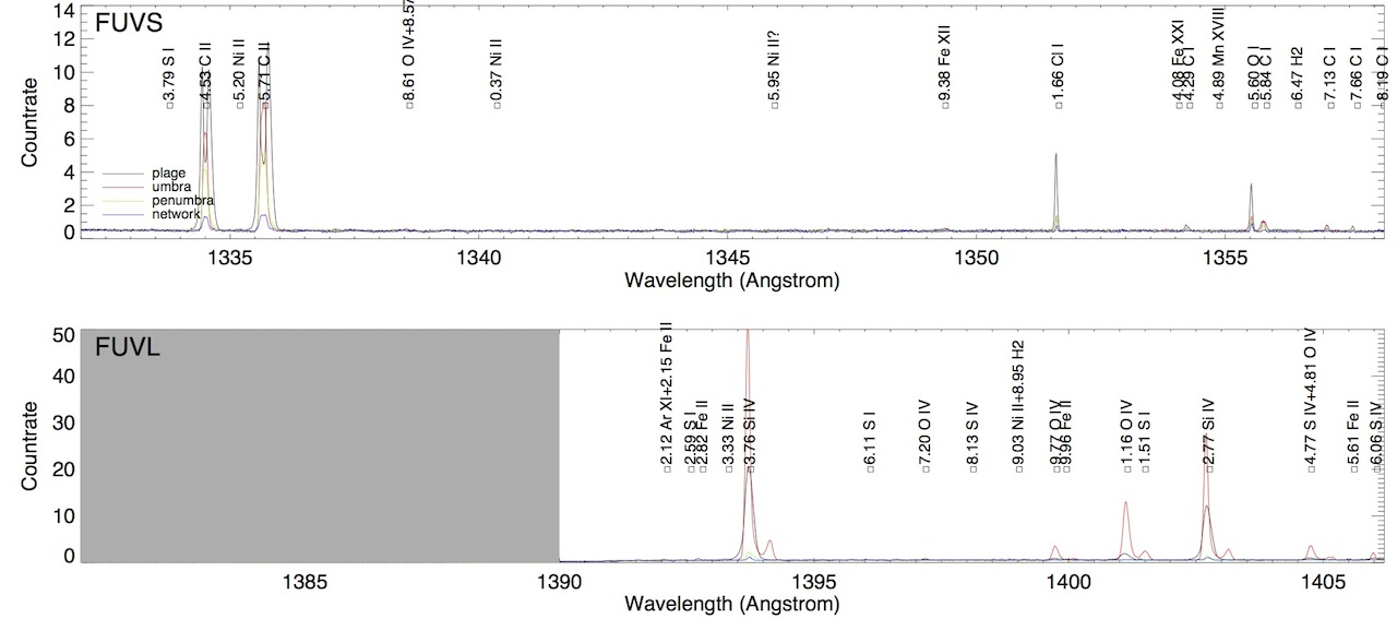
Quiet Sun “FUV” Sample Spectra
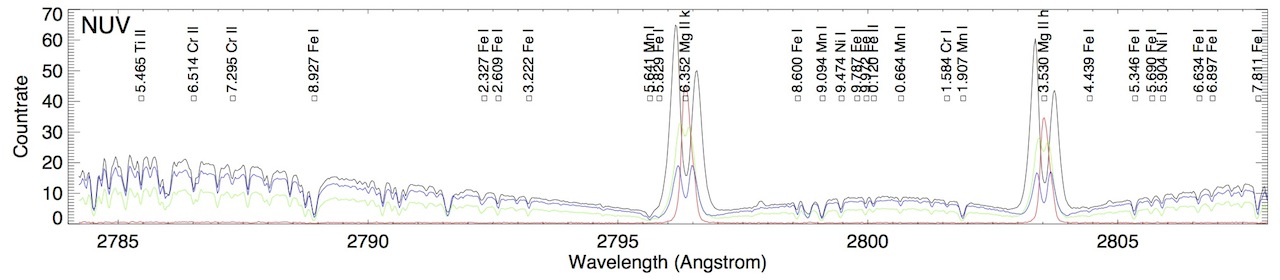
Quiet Sun “NUV” Sample Spectra
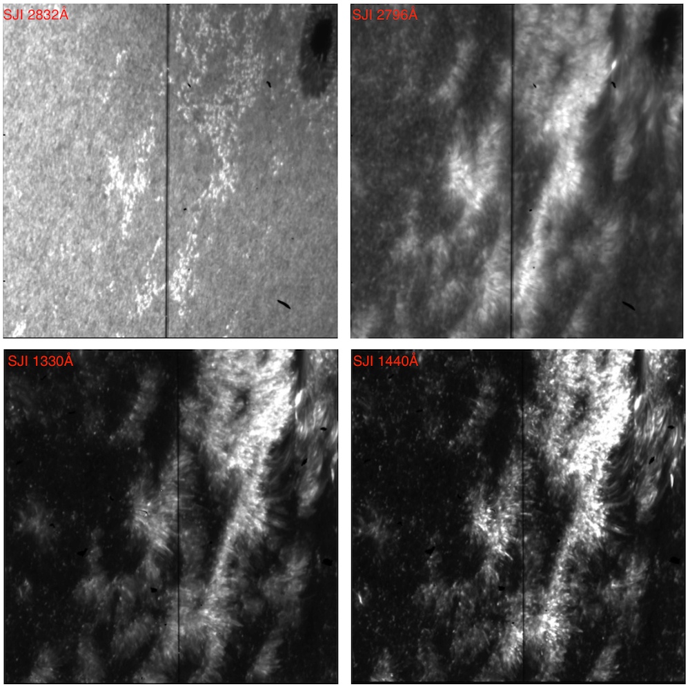
1.4.2. Sample Slit-jaw Images
These sample images taken by IRIS on August 20, 2013 show four of the wavelengths available with the SJI filter selection. Clockwise from the top left is the continuum image in the far red wing of the Mg II k line (“SJI_2832”) and it provides high-contrast photospheric imaging, the Mg II k line (“SJI_2796”) which images the upper chromosphere, the S IV transition region filter (“SJI_1400”), and C II transition region filter (“SJI_1330”). On each of the images note the position of the IRIS SG slit (the dark vertical line) this helps us know that, at that particular time, where the SG slit was placed on the Sun. A preliminary study of the IRIS SJI point spread function (PSF) in the transition region filters indicates that IRIS records the highest resolution images ever taken in the transition region. The SJI images should be flat-fielded to remove small residual CCD artifacts and in the future it will also become possible to deconvolve the point spread function to make the images sharper still (see IRIS Technical Note 29 for further details).
1.5. IRIS IDL routines in SSW
The bulk of the data calibration and analysis routines is written in IDL. Therefore, we recommend that users have a solar soft IDL installation (SSW; http://www.lmsal.com/solarsoft/) to follow this guide. The IRIS branch of the IDL solar soft tree is supported by the mission science team and contains most of the tools you need to handle the data from the instrument FITS files through to manipulating the reduced spectra.
If you have IDL SSW already installed then type the following command upon entering your SSW session to obtain the IRIS package:
IDL> ssw_upgrade, /spawn, /passive, /verb, /iris
To also update the gen folder add , /gen to the IDL command above.
Then, to load the IRIS routines into your path you’ll need to modify the SSW_INSTR environment variable to include them, on UNIX/Mac systems this can usually be found in your .cshrc or .login file:
setenv SSW_INSTR 'iris hessi xrt aia eit mdi secchi sot eis'
On a windows OS this can be modified in your IDL-DE settings/preferences pane.
Warning
The IRIS SSW routines were updated on March 6, 2020 to make them compatible with the latest upgrades of the IRIS data archive. It is therefore essential to update SSW to its latest version.
1.6. IRIS Operations
The observations of IRIS are planned typically for one day (weekdays) or a few days (weekends/holidays). In coordination with the science team, a planner decides on the targets and observing sequences. The resulting work is called a timeline, a list of commands and observing sequences that are run onboard the observatory.
The timeline allows you to see a brief description of each observation along with its “OBS ID” or observing program, the time over which it ran, how many repeats of the sequence were taken, etc. The archive of IRIS timelines can be found online here:
http://iris.lmsal.com/health-safety/timeline/
The timelines are available in 3 formats: TIM, SCI, and GIF. If you choose to download the TIM/SCI file for August 20 2013 and wish to read it, then you can go to the folder http://iris.lmsal.com/health-safety/timeline/iris_tim_archive/2013/08/20/, download the timeline file IRIS_science_timeline_20130820.V00.txt and use the IRIS/SSW routine iris_timeline2struct:
IDL> tl = iris_timeline2struct('IRIS_science_timeline_20130820.V00.txt')
The output of this routine is an array of structures. Each element of the array is a structure describing a single IRIS observing sequence that was run in that time interval:
IDL> help, tl
TL              STRUCT    = -> <Anonymous> Array[23]
IDL> help, tl[0], /str
** Structure <381a378>, 7 tags, length=64, data length=62, refs=2:
DATE_OBS                    STRING          '2013-08-20T04:10:21.000'
DATE_END                    STRING          '2013-08-20T04:11:21.000'
OBSID                       ULONG                   3800
REPEATS                     INT                     10
DURATION                    FLOAT                   6.00000
SIZE                        FLOAT                   9.00000
DESCRIPTION                 STRING          '4 limb coalignment sequence'
The GIF version of the timeline (below) shows graphically how the instrument activities are laid out during the day, the telemetry load, station passes, orbital anomalies (South Atlantic Anomaly – SSA, eclipses, etc). This document provides a detailed legend for the timeline gifs. The timeline GIF for August 20, 2013 is shown below where we can see the characteristics of our sample observation.
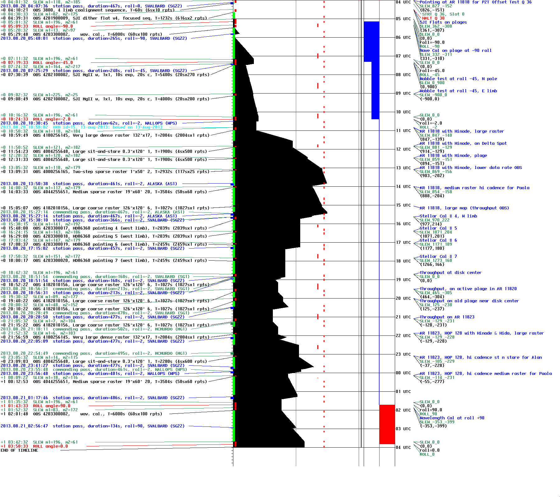
Sample IRIS timeline for August 20, 2013
Alternately, if you want to query the timeline from your IRIS/SSW command line you can use iris_time2timeline, for example:
IDL> t0 = '2013-08-20 00:00:00' & t1 = '2013-08-21 00:00:00'
IDL> tl = iris_time2timeline(t0,t1)
IDL> print, n_elements(tl)
24
IDL> info = get_infox(tl,tag_names(tl),/more)
; Gives a complete report of the observations with the header given by the
; tags of the  timeline structure.
IDL> help, tl[8]
** Structure <3954f18>, 7 tags, length=64, data length=62, refs=2:
DATE_OBS            STRING  '2013-08-20T10:59:49.000'
DATE_END            STRING  '2013-08-20T11:33:12.000'
OBSID               ULONG   4180256145
REPEATS      INT    1
DURATION    FLOAT   2003.70
SIZE                FLOAT   13679.0
DESCRIPTION STRING  'Very large dense raster 132"x175" 400s  C II Si IV Mg II h/k Mg II w s....’
The SSW command struct_where will allow you to search for strings in the description tag which can be useful for finding particular observations:
IDL> ss=struct_where(tl,search=['DESCRIPTION=*coarse*'], program_count)
IDL> help, program_count
PROGRAM_COUNT           LONG      =            5
IDL> print, tl[ss[0]].description
Large coarse raster 126"x120" 64s C II Si IV Mg II h/k Mg II w s Deep x 15 SJI cadence 0.5x
If you are interested in a particular IRIS sequence run over an extended period you can search the timeline structures by OBSID. If we want to identify the number of times the IRIS throughput test sequence (OBSID = 4182010156) was run in August of 2013 then:
IDL> t0 = '2013-08-01 00:00:00' & t1 = '2013-08-30 00:00:00'
IDL> tl = iris_time2timeline(t0,t1)
IDL> through = where(tl.obsid eq 4182010156, count)
IDL> help, count
COUNT           LONG      =           27
1.7. IRIS Documentation and Links
For an in-depth view of the many aspects of the mission, a repository of technical notes built by the science and engineering teams is made available at http://iris.lmsal.com/documents.html. These technical notes (of which the current guide is a part) encompass the areas of Operations, Data Flow, Calibration, Data Analysis, and Numerical Modelling. A list of the different notes can be found below.
In addition to the documentation, below are a few more useful links related to IRIS.
| IRIS Health & Safety Webpage | http://iris.lmsal.com/health-safety |
| IRIS Timelines | http://iris.lmsal.com/health-safety/timeline/ |
| IRIS Technical Note Repository | http://iris.lmsal.com/documents.html |
| IRIS Recent Observations | http://www.lmsal.com/hek/hcr?cmd=view-recent-events&instrument=iris |
| UiO IRIS/Hinode Scientific Data Center | http://sdc.uio.no/sdc/ |
| SUMER UV Spectral Atlas | https://umbra.nascom.nasa.gov/spectral_atlases.html |
| SDO Context Information | http://sdowww.lmsal.com/ |
| Hinode Operations | http://www.isas.jaxa.jp/home/solar/hinode_op/ |
| Hinode/SOT Operations | http://sot.lmsal.com/Operations_new.html |
| Hinode/XRT Operations | http://xrt.cfa.harvard.edu/index.php |