3. IRIS Level 2 Data¶

IRIS Level 2 data can be downloaded from the mission web page or through the European Hinode/IRIS Science Data Center. The IRIS Level 2 files are the calibrated, “science-ready” FITS files distributed to the end-user. The FITS files are designed to allow easy access to the data and metadata; this section describes their structure and typical use cases.

3.1. Structure of IRIS level 2 FITS files¶

The level 2 data are a combination of individual frames for the duration of a given observing sequence (defined by an OBSID number). There are two types of IRIS level 2 files: spectrograph and slit-jaw. The internal structure is different for spectrograph and slit-jaw files, and file naming convention is the following:

Spectrograph: iris_l2_<day>_<time>_<OBSID>_raster_t000_r<raster number>.fits, where <day> is YYYMMDD, <time> is the starting time in HHMMSS, and the raster number starts at zero and up to the total number of raster scans (or repeats) minus one.
Slit-jaw: iris_l2_<day>_<time>_<OBSID>_SJI_<filter>_t000.fits, where <filter> is the filter central wavelength in Å (1330, 1400, 2796, or 2832).

The number of spectrograph files depends on the type of observing sequence. For sit and stare or single-raster programs (e.g. 400-step raster) there is only one file. For multiple-repeat rasters, there is one file per raster scan. Data from both FUV and NUV detectors are combined in each file. The FITS structure comprises one primary Header-Data Unit (HDU) and several extensions. The primary HDU contains no data, only a header. The science data are saved in the subsequent extensions (one extension per spectral window), and additional metadata are saved in the last two extensions.

For slit-jaw files there is only one file per filter per observing sequence. The FITS structure comprises one primary Header-Data Unit (HDU) and two extensions. The science data are saved in the primary HDU, while additional metadata are saved in the first and second extension.

The tables below illustrate the HDU structure for slit-jaw and spectrograph files.

Structure of level 2 spectrograph files. `nwave_n` denotes number of wavelength points in spectral window n. `ny` denotes number of spatial Y points. `nrt` denotes number of raster positions (multiple raster programs) or number of time positions (sit and stare programs).¶
HDU #	HDU type	Contents	Data dimensions
0	Primary	Main header	No data
1	Image Extension	Data for wavelength window 1	[`nwave_1`, `ny`, `nrt`]
2	Image Extension	Data for wavelength window 2	[`nwave_2`, `ny`, `nrt`]
…
n	Image Extension	Data for wavelength window n	[`nwave_n`, `ny`, `nrt`]
n + 1	Image Extension	Auxiliary metadata	[47, `nrt`]
n + 2	Table Extension	Technical metadata	[`nrt`, 7]

Structure of level 2 slit-jaw files. `nx` denotes number of spatial X points. `ny` denotes number of spatial Y points. `nt` denotes number of time positions.¶
HDU #	HDU type	Contents	Data dimensions
0	Primary	Main header and data	[`nx`, `ny`, `nt`]
1	Image Extension	Auxiliary metadata	[30, `nt`]
2	Table Extension	Technical metadata	[`nt`, 5]

A description of the level 2 keywords, for primary and extension headers, is available for download.

The auxiliary metadata contain several quantities for each exposure. These are parameters that may vary for different exposures and are therefore stored here. The header of this HDU gives the different keywords and their index in the table. For example, TIME has the value 0, meaning that data[0, *] will give an array with the times of each exposure, for all timesteps or raster steps.

Note

In case of missing exposures, most of the parameters in the auxiliary metadata are set to 0. There are some exceptions: DSRCFIX, DSRCNIX, and DSRCSIX are set to -1. Some auxiliary metadata values are not given for both NUV and FUV detectors. In such cases, the values are taken from the FUV source file, and if the FUV file is missing they are taken from the NUV file. If both NUV and FUV source files are missing, the parameters are set to 0. Exceptions are TIME, which is set to the planned time of the respective exposure, and PZTX and PZTY, which are set to the minimum value of all PZTX and PZTY values, respectively, within the particular fits file. The following parameters are not separate for FUV and NUV: TIME, PZTX, PZTY, XCENIX, YCENIX, OBS_VRIX, OPHASEIX, PC1_1IX, PC1_2IX, PC2_1IX, PC2_2IX, PC3_1IX, PC3_2IX, PC3_3IX, PC2_3IX.

The technical metadata in the last extension are usually not useful for the end-user. Their content is only useful for reproducing the exact steps of the data calibration, and contain details such as FRM, FDB, and CRS IDs, names of level 1 files used. The header of the last extension contains some information about the format.

3.2. Searching and Downloading¶

3.2.1. Using the IRIS Data Search Webpage¶

The IRIS data search webpage (http://iris.lmsal.com/search) is designed to quickly guide researchers to IRIS datasets appropriate for their research. It consists of five graphical elements and three steps to the data:

IRIS Banner
Selection widgets
Graphical display of search results on a solar image
Tabular display of search results
Dataset browser/inspector with links to download the data sets

The IRIS data search tool is optimized for use on landscaped displays of at least 1280x768 pixels. The banner and the solar image can be hidden (displayed) by clicking on the red (green) buttons in the upper left corners to accommodate smaller screens. The tool has been tested with recent versions of Firefox, Safari and Chrome browsers. If you have difficulty with the tool, you might first try one of these browsers to ensure compatibility.

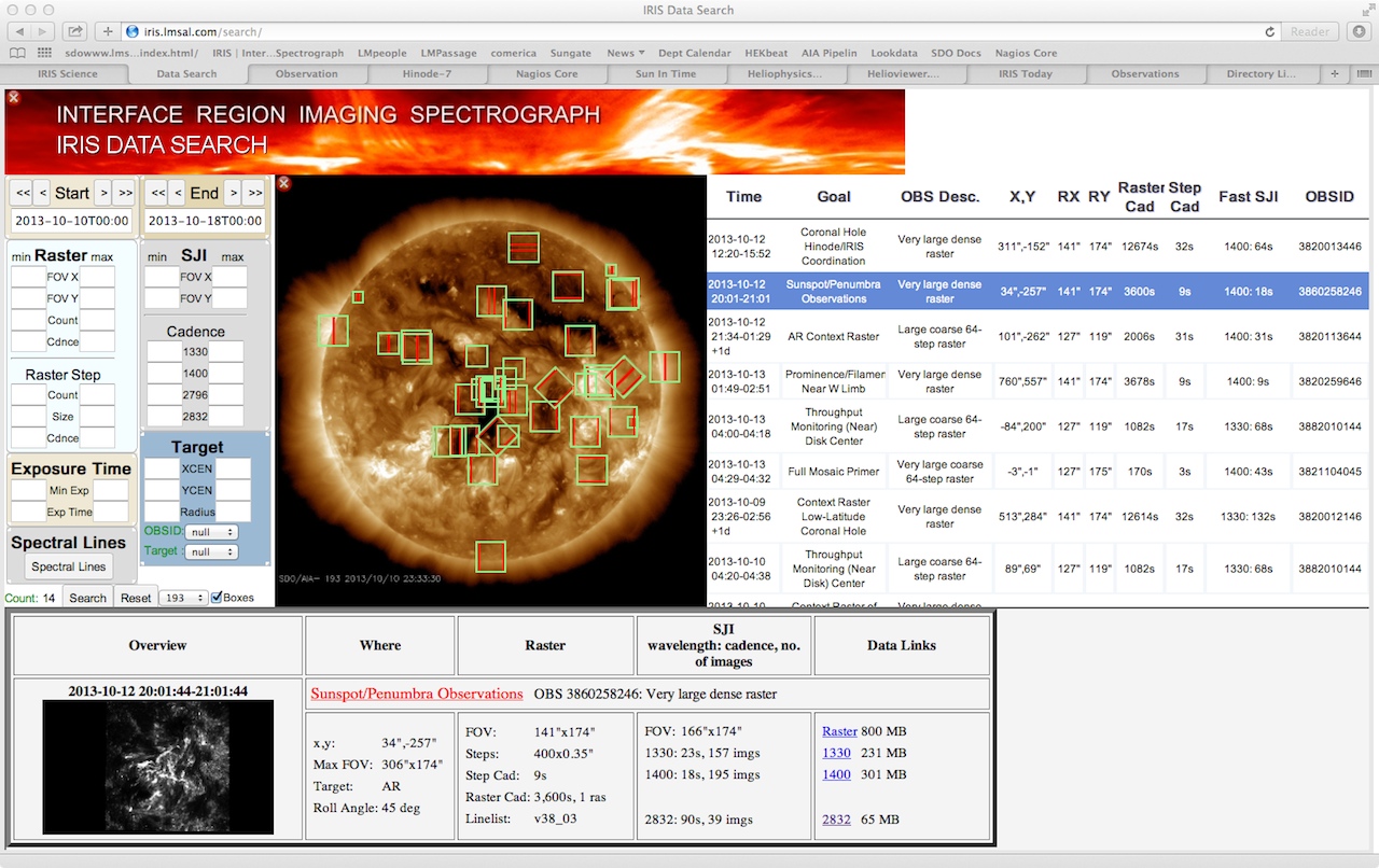
IRIS search sample screenshot

Selection widgets: There are six widgets available for customized, dynamic, data searches. At the most basic this search consists of specifying the start and end of a time range of interest. When first loaded these default to select the week surrounding the current date. The start and end times can be moved forward and back a day or a week by using the single and double arrow buttons. Specific dates can be entered directly into the text boxes or by using the calendars that popup when one clicks on them. The total count of datasets available within the time range appears at the bottom left of this selection area. By default, only datasets that are completely processed are displayed. If you wish to include ones that are still processing, uncheck the only OBS with data box below count (not shown in figure).

The remaining widgets are used to filter the selections within the specified time range. The count of available data sets updates dynamically to reflect the effects of your selections.

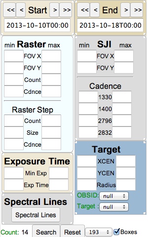
IRIS search selection widgets

Raster: Limit results to datasets with rasters within a (min, max) range of: fields of view in arcseconds; number of repeats (count); and of the cadence in seconds and with raster steps within a range of number (count); size in arcseconds and cadence in seconds.

Slit Jaw Imager (SJI): Limit results to datasets with slitijaw images within a range of fields of view and cadences for each wavelength band.

Exposure time: Limit results to datasets within a range of minimum exposure and mean exposure times based on all images within the dataset.

Target: Limit results to a range of target positions relative to disk center in arcseconds either as a bounding box (xcen, ycen) or an annulus between radii. Limit sets to specific IRIS Observation IDs or target. The colors of these last two change to indicate the presence (green) or absence (red) of matching datasets based upon other selections.

When all selections are made, clicking the search button refreshes the results in the display area. Note that the display does not update while you are constructing a search. A range of background SDO/AIA images of the sun corresponding to the start time of query can be selected for the display. All filters (other than dates) and displays are cleared by clicking the reset button.

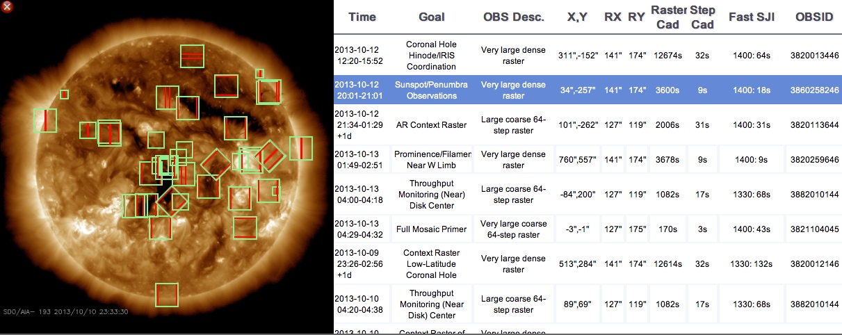
IRIS search display widget.

Display Widget: The results of a search are displayed on a co-temporal AIA image that is selectable from the search widget. The default setting displays the bounding boxes for the slit jaw (raster) image as green (red) rectangles on an 193 Å AIA image. A sortable list of IRIS observations on the right presents details of the dataset including the time interval, short descriptions, pointing, fields of view, cadences and observation IDs. Clicking on an entry in either widget, highlights the selection in the table along with a detailed description in the inspection widget.

IRIS search inspection widget

The latest version of the search engine includes the option to find all IRIS observations for which co-aligned SDO and/or Hinode data cubes are available. This can be done by checking the appropriate option buttons located under the “More” button.

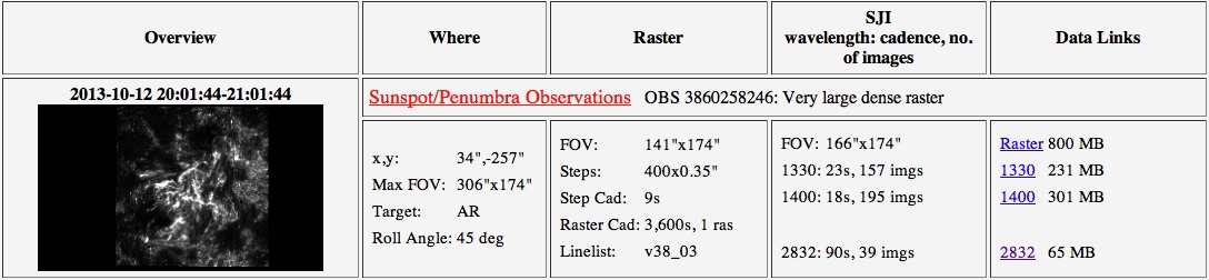
Inspection Widget: The inspection widget shows more details of the dataset, including a thumbnail slitjaw image, pointing information and links to and sizes of the data products (when they become available). Clicking on the image or title will bring up a separate details page with summary movies, paths to the data and links to the AIA cutout service. Clicking on the data links will immediately download the corresponding gzipped dataset.

3.2.2. Using SSW IDL¶

IRIS Level 2 data can be accessed via the SSW command line using a simple extension of the IDL/SSW timeline queries used above. So, our earlier example:

IDL> t0 = '2013-08-20 00:00:00' & t1 = '2013-08-21 00:00:00'
IDL> tl = iris_time2timeline(t0,t1)
IDL> info = get_infox(tl, tag_names(tl), /more)

returns the details of all IRIS observations taken on August 20, 2013. If we want to browse those sequences with OBSID = 4182010156 then we can use the following command to return the location of the IRIS Level 2 data for each relevant sequence:

IDL> hcr = iris_time2hcr(t0,t1,/expand_eventid,limit=2000,/struct)
IDL> fg=where(hcr.obsid eq '4182010156')
IDL> l2_folder = str_replace(hcr[fg].url,'/level2/','/level2_compressed/')
IDL> print, l2_folder
http://www.lmsal.com/solarsoft/irisa/data/level2_compressed/2013/08/20/20130820_150507_4182010156/
http://www.lmsal.com/solarsoft/irisa/data/level2_compressed/2013/08/20/20130820_185222_4182010156/
http://www.lmsal.com/solarsoft/irisa/data/level2_compressed/2013/08/20/20130820_194022_4182010156/
http://www.lmsal.com/solarsoft/irisa/data/level2_compressed/2013/08/20/20130820_201022_4182010156/
http://www.lmsal.com/solarsoft/irisa/data/level2_compressed/2013/08/20/20130820_211522_4182010156/

The www subfolder in each example contains a collection of browsable movies of the slit-jaw and spectrograph image sequences taken during the observation like that shown below. These movies can be used to view the data before downloading the (large) Level 2 FITS files.

Browsable movies from data webpage.

Extending this example to a more specific case let’s pick the first of these OBSID = 4182010156 observations and recover the URLs for the IRIS Level 2 FITS files from the command line:

IDL> tmp = where(tl.obsid eq 4182010156)
IDL> tl = tl[tmp[0]]
;raster files
IDL> l2_rasters=iris_time2files(t0, t1, obsid = 4182010156, /raster, level=2, /urls, /compressed)
IDL> help, l2_rasters
L2_RASTERS         STRING    = Array[5]
IDL> print, l2_rasters
http://www.lmsal.com/solarsoft/(...)/iris_l2_20130820_150507_4182010156_raster_t000_r00000.fits
http://www.lmsal.com/solarsoft/(...)/iris_l2_20130820_185222_4182010156_raster_t000_r00000.fits
http://www.lmsal.com/solarsoft/(...)/iris_l2_20130820_194022_4182010156_raster_t000_r00000.fits
http://www.lmsal.com/solarsoft/(...)/iris_l2_20130820_201022_4182010156_raster_t000_r00000.fits
http://www.lmsal.com/solarsoft/(...)/iris_l2_20130820_211522_4182010156_raster_t000_r00000.fits
;SJI files
IDL> l2_sji=iris_time2files(t0, t1, obsid = 4182010156, /sji, level=2, /urls, /compressed)
IDL> help, l2_sji
L2_SJI         STRING    = Array[20]
IDL> print, l2_sji
http://www.lmsal.com/solarsoft/(...)/iris_l2_20130820_150507_4182010156_SJI_1330_t000.fits
http://www.lmsal.com/solarsoft/(...)/iris_l2_20130820_150507_4182010156_SJI_1400_t000.fits
...
http://www.lmsal.com/solarsoft/(...)/iris_l2_20130820_211522_4182010156_SJI_1400_t000.fits
http://www.lmsal.com/solarsoft/(...)/iris_l2_20130820_211522_4182010156_SJI_2796_t000.fits
http://www.lmsal.com/solarsoft/(...)/iris_l2_20130820_211522_4182010156_SJI_2832_t000.fits

Naturally these files could have been viewed by opening the web folder found earlier. These L2 FITS files can be downloaded to your local folder using a web browser or by using the SSW command:

;raster files
IDL> sock_copy, l2_rasters, out_dir='./'
;SJI files
IDL> sock_copy, l2_sji, out_dir='./'
IDL> $gunzip *fits.gz
IDL> $ls *.gz |xargs -n1 tar -xzf

Once the files are finished downloading you are ready for the next step - read them or use our tools to dig a little deeper.

3.3. Browsing Level 2 Data with `iris_xfiles`¶

One way to browse and manipulate Level 2 IRIS data is to use the widget routine iris_xfiles. This routine is run from the IDL command line as follows:

IDL> iris_xfiles

The iris_xfiles interface appears as below. The search directory window will let you browse your IRIS data directory tree. But in this case it is better to remove the file search filter so that you can see where you are navigating. When navigating double click on a directory name in order to enter the directory.

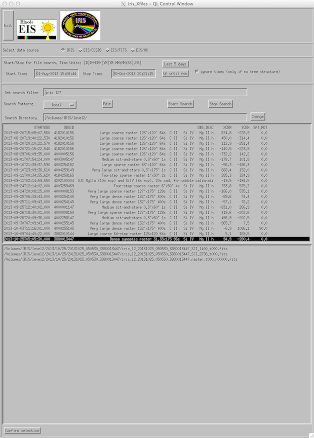
IRIS_xfiles main interface.

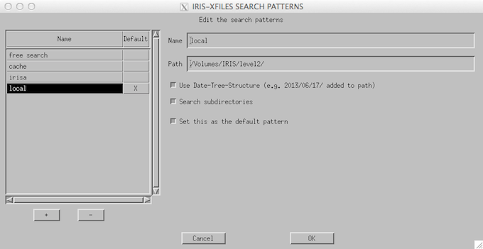
If the user is downloading Level 2 FITS files on a locally mounted drive (like the example we show here) then the user should edit the “search pattern” tab (below) to the folder in which the IRIS Level 2 FITS files are contained. Click on the edit button to change the configuration.

IRIS_xfiles file picker.

Level 2 FITS files of two types can be picked from the file picker: iris_l2*SJI*.fits & iris_l2*_raster_*.fits which, as we have discussed above, contain the slit jaw images in a given filter taken during an observing sequence, or the spectral images of an observing sequence, respectively.

Selecting one of the slit-jaw raster FITS files - by clicking on Confirm Selection, or just double-clicking the file - will bring up the widget called iris_ximovie. iris_ximovie (which can also be used individually on FITS data loaded at the command line) allows the user to view the slit jaw sequence as a movie. It contains a number of options for playback speed, change of magnification, zooming, blinking, and the generation of postscript, jpeg or gif output as well as MPEG movies through the “file/save_as menu”.

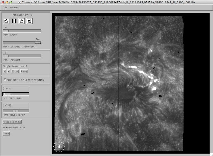
iris_ximovie widget.

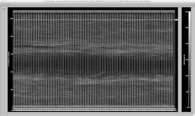
iris_xfiles can multi-task so you can have multiple analysis/movie/widget windows open simultaneously while you study your data. So, selecting the raster FITS file you will see the following X11 window pop up, the iris_xcontrol widget. In this case the requested raster is read, as are the available slit jaw images that were taken during this particular raster.

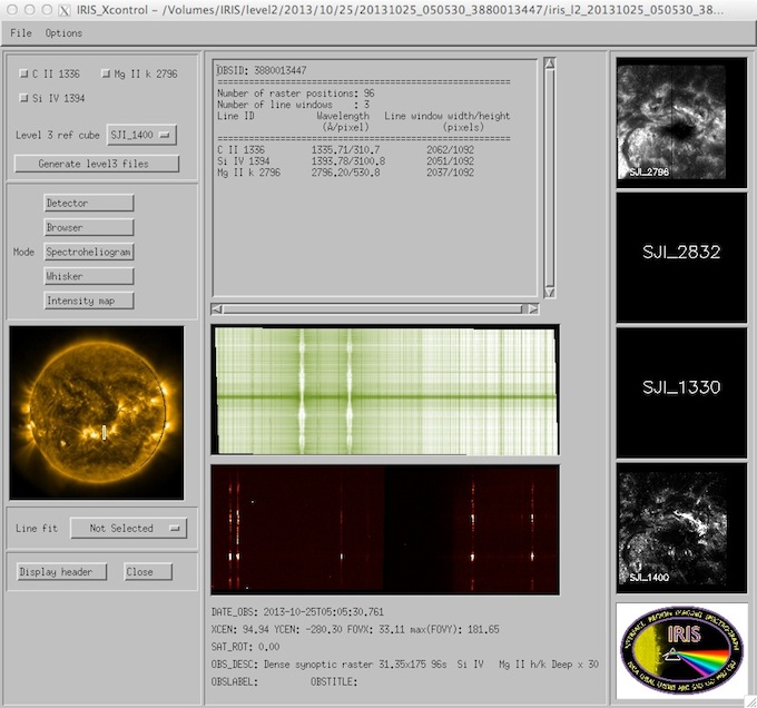
iris_xcontrol main interface.

iris_xcontrol (above) is the main control widget for the IRIS L2 quicklook software. It launches an array of other QL widget programs.

An overview of the raster is given in the middle top window that includes the OBSID, the number of raster positions, the number of spectral (line) windows, their wavelength and pixel ranges on the IRIS CCDs as well as their name - the names are usually associated with the principal spectral line in the window. Many of the other quicklook widgets driven by iris_xcontrol require a line list given by this selectable list. The “Generate Level 3 files” button of iris_xcontrol will generate a set of Level 3 files for analysis like CRISPEX.

The left of the iris_xcontrol widget is an SDO/AIA 171Å image of the Sun taken closest in time to the start of the observation. The location of the IRIS scan or sit-and-stare observation on the Sun is shown as a box or a vertical line respectively. The image, if found, should be current in the sense that it is taken on the same day as the raster. Right clicking on the solar image will toggle between various AIA images. Left clicking will bring up a widget containing a magnified copy of the image including the raster pointing.

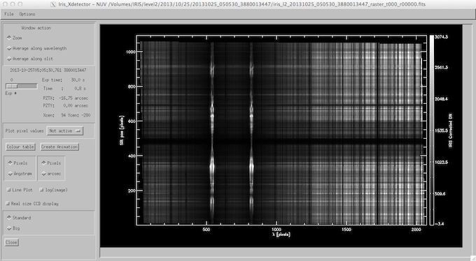
iris_xdetector widget.

The lower middle window of iris_xcontrol show the layouts of the spectral windows (or regions) on the NUV (top) and FUV (bottom) CCDs. The lower window shows the combined FUV1 and FUV2 CCDs (see the introduction for further information). Clicking on these windows will start the “Detector” quicklook widget (below) which shows the layout of the spectral windows on the CCDs with options to cycle through the exposures of the raster, plot/print pixel values, change the color table, etc. This widget can also be started by clicking on the “Detector” button, which can be found just above the AIA image window. The “Create Animation” button in the Detector widget often provides a very interesting movie of the spectral evolution during the observation - particularly for sit-n-stare observations.

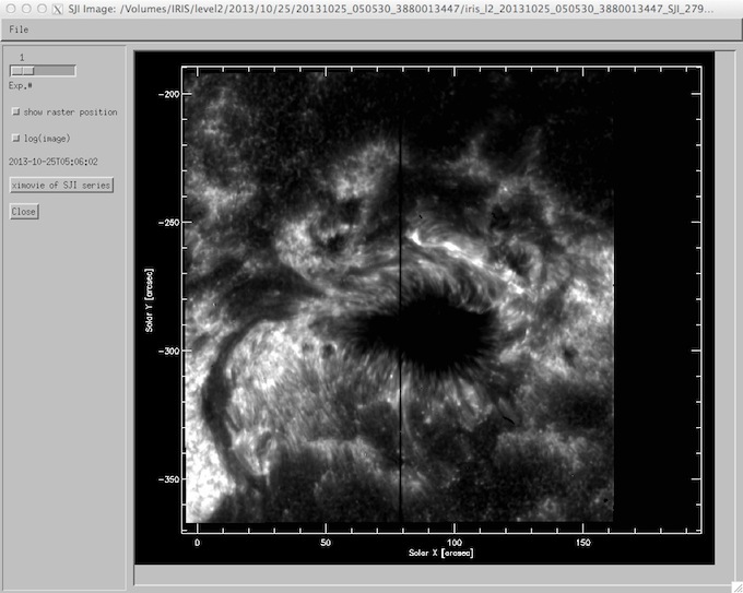
The right column of iris_xcontrol shows up to four slit jaw images taken during the raster. Clicking on any of these will bring up a widget (iris_sji_image; see below) containing a magnified image of the slit jaw, sliders to cycle through the slit jaws taken during the raster, and the option to plot the location of the raster exposures taken (compare with iris_ximovie). An instance of ximovie can be started for the SJI sequence by clicking on the button.

iris_sji_image widget.

Below the “Detector” button on iris_xcontrol - in the center of left column - are the buttons for starting the “Browser”, the “Spectroheliogram”, “Whisker” and “Intensity Map” widgets.

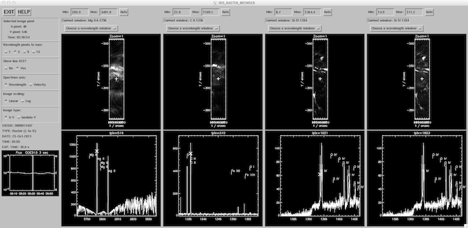
iris_xfiles browser.

Browser: The “Browser” is similar to the Hinode/EIS quicklook browser tool (above), and has recently been modified for IRIS. We note that the browser routine (iris_raster_browser) can run independently of iris_xfiles by calling:

IDL> iris_raster_browser, l2f
; where l2f can be an IRIS data object or a Level 2 FITS file

Spectroheliogram: Selecting one or more line windows in the upper left panel of iris_xcontrol and clicking the “Spectroheliogram” button will bring up a widget that contains images of the spectral windows taken during the raster (see below). The spectral movie strips are arranged vertically according to line window and horizontally according to exposure number. Options in the spectroheliogram widget include setting the spectra on pixel or Å wavelength scales and/or pixel or arcsec.

iris_xfiles spectroheliogram.

Whisker: Select one (or more) spectral windows in order to view the windows arranged according to raster position (or exposure number) at a given slit position. This is a widget that presumably is best used for “sit and stare” type observations where one can follow the time evolution of a given location on the sun in a specific spectral line.

Intensity: The “Intensity Map” function of iris_xfiles is very powerful and will integrate the selected spectral windows over a given range of wavelengths and display the result as an image (see below). This is an excellent tool for examining the wing behavior, or the properties of the complex Mg II h &k (below and left) lines or the C II 1330Å lines.

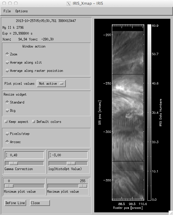
iris_xfiles intensity map.

By default “Intensity” will integrate over the entire spectral window chosen. However, by clicking on the “Define Line” button parts of the spectral line (or the continuum) can be chosen for integration and presentation in the image window. When “Define Line” is pressed a small widget is brought up (see below) where one can define properties such as the “line start” and “line stop” locations. The integration of the line intensity is done between these locations. Furthermore, when the “Continuum Start” and “Continuum Stop” sliders are used “Intensity” will compute an average intensity of the continuum that is then subtracted from the line intensity integral. The example shown above (for the Mg II h line) shows an image of the integrated core reversal wing minus a small continuum patch in the red wing.

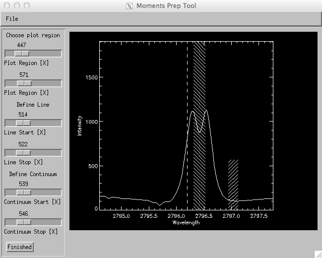
Define line dialong for intensity map or profile moments.

As with the other tools there are options to zoom in on the images, plot pixel values, change color tables and gamma factors in the images, swap between pixel and arcsec spatial scales, etc.

The “Line Fit” gadget: The Line Fit gadget on the iris_xcontrol interface can perform rudimentary spectral analysis of the optically thin FUV lines. It can also be used to inspect the optically thick Mg II and C II lines, but the analysis required for these lines is significantly more complex than this tool permits (see chapter on IRIS Level 3 Data).

The “Profile moments” pull down menu will do simple calculations of line moments (see below), either directly or via Gaussian fits to the selected lines. The results of these calculations will be displayed with the Intensity map tool, now with the possibility of choosing whether to view intensities, velocities, widths, or continuum intensities.

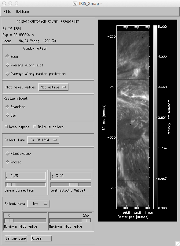
Profile moments dialog.

Running with “moments” is relatively straightforward. This will compute the zeroth (intensity), first (doppler velocity), and second (line width) moments of the intensity profile. First, the “define line” window will pop up, once for each line checked off in the “select line” pane. Thereafter, the “intensity map” tool will pop up with some extra options for displaying the intensity, velocity, or line width of the various lines chosen. The image can be resized, with or without the aspect ratio being retained. The height of this image is the same as that produced by the slit jaw viewer (“xsji_image”) so the images should be directly comparable.

3.4. Reading Level 2 Data in IDL¶

3.4.1. Using The IRIS Level 2 Data Object¶

The IRIS level 2 software is designed to allow the user to easily read and access the data and keywords contained in IRIS level 2 fits files. It is also designed to be used by the IRIS QL software, i.e. those widgets called by iris_xfiles. The software is made up of several objects; iris_data, iris_aux, iris_sji, iris_cal, iris_moment, etc, the most important of which is by far the iris_data object. The casual user does not have to worry too much about this, at least not initially. The following are examples that show how to read the fits file header, load an IRIS raster window (region) into memory, as well as locate important auxiliary information.

To construct an iris_data object one first needs to find a set of iris files. Go to a directory that contains iris files, or make a text variable “path” that contains the path to iris files. The function iris_files will load in selected iris files:

IDL> f = iris_files(path=path)

returns the list of fits files in the directory path (default './') and prints this list on the screen. Then, assuming that f[X] is a level 2 iris raster file:

IDL> d = iris_load(f[X])

This populates the data object with the fits header, auxiliary information, and (pointers to) the data itself. You can get help on the data object and its methods with:

IDL> d.help
Class: IRIS_DATA
file: /opt/solarsoft/iris/idl/uio/objects/iris_data__define.pro
version: $Id: iris_data__define.pro,v 1.114 2017/05/22 09:23:23 mawiesma Exp $
FUNC init,file,verbose=verbose                                    : initializes object, calls read if "file" parameter given
PRO  close                                                        : frees pointer to main data array "w" and closes all associated files
PRO  cleanup                                                      : called by obj_destroy, frees all pointers and closes all associated files
PRO  help, description=description                                : prints out this help, setting the 'description' keyword will also print the header info
FUNC getfilename                                                  : returns the raster filename
FUNC getfilename_sji,lwin                                         : returns the sji filename of lwin (lwin=0 through 5)
FUNC getcomment                                                   : returns comment for object
PRO  setcomment,comment                                           : sets comment for object
FUNC getaux                                                       : returns the aux data as an iris_aux object
FUNC getcal                                                       : returns IRIS specific parameters as an iris_cal object
FUNC missing                                                      : returns the "missing" value
FUNC getnwin                                                      : returns the number of line windows
(...)

Here we detail some of the available methods. For example, to retrieve the fits header:

IDL> hdr = d->gethdr(iext, struct=struct)

The function gethdr takes a parameter iext (default 0) which gives the extension to be displayed (remember that the level 2 fits files have a main header “0” and one header for each line window or region). There is one keyword, /struct which when set, return the header as a IDL structure instead of a string array. Or if one wants to look at a specific keyword tag:

IDL> print, d->getinfo('tag')

will produce it. In addition to tag this function takes another parameter iext (default 0) and a keyword sji such that /sji will return the value of the keyword tag in slit jaw header iext.

A very useful procedure is:

IDL> d->show_lines
Spectral regions(windows)
 1335.71   C II 1336
 1349.43   Fe XII 1349
 1351.17   1351
 1355.60   O I 1356
 1393.78   Si IV 1394
 1402.77   Si IV 1403
 2786.52   2786
 2796.20   Mg II k 2796
 2831.33   2831
Loaded Slit Jaw images
 SJI_1330
 SJI_1400
 SJI_2796

which gives an overview of the line(s) and SJI windows loaded into the object. This function only works on raster FITS files, not SJI FITS files.

To actually look at the data, use:

IDL> win = d->getvar(iwin, load=load)

to get data for window number iwin. The win variable now contains a three dimensional array win[lambda, ypos, xpos and/or exposure nr]. The data is by default returned as a pointer to a location in the fits file and that access to the data therefore is through the IDL assoc mechanism. That is:

IDL> dum = win[*,*,12]

or:

IDL> dum = (d->getvar(iwin))[*,*,12]

will contain the 12th exposure (raster position) of window iwin.

If one requires the entire window to be read into memory instead of looking at one exposure at a time, a /load option should be passed to getvar:

IDL> win = d->getvar(iwin, /load)

Note that the /load option will also descale the data (using the descale_array method). At this point you may decide that you have had enough of objects. “Just give me the data”:

IDL> s = d->getdata()

Will return a structure that contains the “entire” object, along with various auxilary information. Note that IRIS level 2 files can be quite large, so do not use this method uncritically. Note that reading in data to the structure may take some time.

For those sticking with objects, the wavelength lambda for window iwin is given by:

IDL> lambda = d->getlam(iwin)

where iwin can be either the window number or the approximate wavelength of the window (the software will find the window if the wavelength given lies inside the wavelength range of the spectral window).

The slit position (y) is given by:

IDL> y = d->getypos()

The method getypos takes an iwin argument, but all windows share the same y-scale so it is not necessary to specify it. The raster (x) and/or time (t) coordinate are found via:

IDL> x = d->getxpos(iwin=iwin)
IDL> t = d->gettime()

The time returned is relative to STARTOBS, note that you can also get the absolute time via:

IDL> tai=d->ti2tai()    ; Atomic time in seconds
IDL> tutc=d->ti2utc()   ; UT

Here is a simple IDL script that shows how this can be done avoiding objects all together (the script can be found in the “utils” directory of the SSW distribution):

iris_readheader,f,struct=struct,extension=extension
    if n_elements(extension) eq 0 then extension=0
    d = iris_obj(f)
    hdr = d->gethdr(extension,struct=struct)
    obj_destroy, d
    return, hdr
end

The gethdr method by default will return the main (extension=0) fits header, but since the various IRIS line windows (regions) are stored as extensions 1, …, NWIN, there is a small header associated with each which may be useful. Using the struct keyword will return the header as an idl structure instead of a string array. In the latter case header tags (keywords) can be accessed with the usual SSW fxpar(hdr, tag) routines. Note that since the main header is contained in extension=0, the window headers are accessed as extension=window nr + 1.

In general, this should be the recipe for writing small “one-liners”:

open and load the object, viz d = iris_obj()
call the methods needed to do what you want to do
manipulate and make the output available
destroy the object

Other examples (of many, see below) are:

IDL> exp = d->getexp(iexp, iwin=iwin)

or:

IDL> xpos = d->getxpos(indx, iwin=iwin)

to get the exposure time for exposure number iexp or spatial index indx in window number iwin. These functions return an array of exposure times or spatial positions if no parameter iexp or indx is given, and default to the default window (the first one read) if no iwin keyword is given.

To check the data integrity and returned structures:

IDL> s = d->aux_info() ; extension nwin+1
IDL> s = d->obs_info() ; extension nwin+2

The help command can be used to view their content:

IDL> help, s ; will show their content.

There are a number of objects that are detailed in IRIS Technical Note 28 as well as a list of other methods that can be applied to the data.

3.4.2. Using `read_iris_l2.pro`¶

IRIS Level 2 FITS files can be read into memory using the read_iris_l2 procedure:

read_iris_l2, l2files, index, data, _extra=_extra, keep_null=keep_null, $
          append=append, silent=silent, wave=wave, remove_bad=remove_bad

where l2files can be an array of Level 2 FITS files. The wave keyword can be used to select a specific wavelength window (e.g., wave = 'Si IV 14') for a raster FITS file. The option has no impact on SJI FITS files. An example call to read_iris_l2 to read an SJI Level 2 FITS file:

IDL> sjifile = 'iris_l2_20131025_050530_3880013447_SJI_1400_t000.fits'
IDL> read_iris_l2,sjifile, index, data
IDL> help, index, data
INDEX           STRUCT    = -> <Anonymous> Array[48]
DATA            FLOAT     = Array[1214, 1092, 48]
IDL> rastfile = 'iris_l2_20131025_050530_3880013447_raster_t000_r00000.fits'
; define the object (see below) - convenient way to show spectral windows
IDL> d = iris_obj(rastfile)
IDL> d->show_lines
Spectral regions(windows)
0   1335.71   C II 1336
1   1393.78   Si IV 1394
2   2796.20   Mg II k 2796
IDL> read_iris_l2,rastfile,index,data, WAVE= 'C II' ; default C II
; other WAVE options in this IRIS line list would be 'Si IV', or 'Mg II'
; NOTE: often there is more than one Si IV and one can extend to the
; string to make it unique
; 'Si IV 13' or 'Si IV 14'
IDL> help, index, data
INDEX           STRUCT    = -> <Anonymous> Array[96]
DATA            FLOAT     = Array[2062, 1092, 96]

where, naturally index and data are arrays that contain the header information for each raster step and the corresponding spectrograph data.

Using IDL procedure iris_prep_version_check.pro, we can check whether the fits files are for the most recent processing, i.e., calibration:

IDL> calcheck=iris_prep_version_check(index, /loud)

or:

IDL> calcheck=iris_prep_version_check(l2file, /loud)

where index is a fits header and l2file is an IRIS level2 fits file (with full path). For this particular example we can therefore run the following command:

IDL> calcheck=iris_prep_version_check(index, /loud)

here calcheck is a boolean function, which returns 1 if current data is good, while 0 implies that the fits files should be downloaded again since calibration procedure was improved in the meantime and updated fits files are available. The keyword /loud prints extra info when set.

3.5. NUV Data Analysis¶

3.5.1. Mg II Diagnostics¶

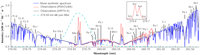
In the following sub-sections we’ll document a couple of methods to extract physical information from the IRS NUV spectra. These optically thick lines are typically tough to interpret but the IRIS team has done some exploratory work to help the community get as much from the data as possible. The singly ionized Mg II h&k lines (http://adsabs.harvard.edu/abs/1997SoPh..172..109U) provide information that spans from the photosphere to the upper chromosphere (and possibly as high as the transition region).

The image below shows a comparison synthetic and observed Mg II spectra adapter from the paper by Pereira et al. (2013) The h and k emission cores are typically double-peaked - and can be characterized on the violet ‘V’ or red ‘R’ side of the rest wavelength - see the inset.

IRIS Technical Note 37, as well as the three IRIS diagnostic papers from the ITA/UiO team:

provide a comprehensive review of how these parameters can be interpreted in terms of the Bifrost simulations (see IRIS Technical Note 33). The interested IRIS user should consult these papers before studying FUV data in detail. The table below gives a summary of the basic physical properties that can be extracted from the Mg II h&k lines, the bonus being that having two lines that there is some level of comfort in getting consistent measures.

Spectral observable	Atmospheric property
\(\Delta v_{k3}\) or \(\Delta v_{h3}\)	upper chomospheric velocity
\(\Delta v_{k2}\) or \(\Delta v_{h2}\)	mid chromospheric velocity
\(\Delta v_{k3} - \Delta v_{h3}\)	upper chromospheric velocity gradient
\(k\) or \(k\) peak separation	mid chromospheric velocity gradient
\(k_2\) or \(h_2\) peak intensities	chromospheric temperature
\((I_{k2v}-I_{k2r}) / (I_{k2v}+I_{k2r})\)	sign of velocity above \(z(\tau=1)\) of \(k_2\)

Note

The above table shows a simplified view, and all the correlations have scatter.

The codes discussed below provide measures of these properties and a few others.

3.5.2. Mg II Line Peak Information Extraction¶

Tiago Pereira (ITA/UiO) has developed a piece of IDL software which will permit IRIS users to extract properties of the Mg II h&k lines in the NUV spectra. The code, when given an IRIS Level 2 data file, will return the properties of the red peak, blue peak and central reversals of the Mg II h&k line spectra based on a relatively straightforward peak finding algorithm.

The code, iris_get_mg_features_lev2 is executed in the following way:

IDL> myfile = 'iris_l2_20131013_090250_3821104045_raster_t000_r00000.fits'
IDL> d = iris_obj(myfile)
; Find the index of the Mg II window:
IDL> d->show_lines
Spectral regions(windows)
0   1335.71   C II 1336
1   1349.43   Fe XII 1349
2   1355.60   O I 1356
3   1393.78   Si IV 1394
4   1402.77   Si IV 1403
5   2832.75   2832
6   2814.47   2814
7   2796.20   Mg II k 2796
IDL> vr = [-40, 40] ; Velocity Range about line center to search for features
IDL> iris_get_mg_features_lev2, myfile, 7, vr, lc, rp, bp

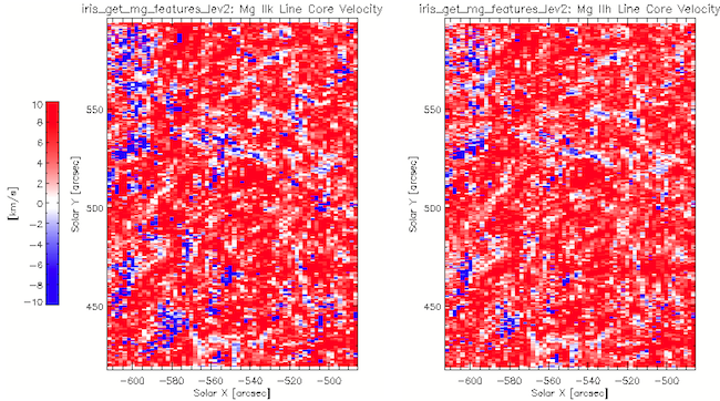
Sample Mg II h/k velocities obtained with iris_get_mg_features_lev2.

In this example the results are stored in the lc, rp, bp arrays corresponding to the central reversal, red and blue peaks respectively. Each of these arrays is organized [line, feature, slit position, raster position]. The line index corresponds to Mg II k [0] and Mg II h [1]. The feature index corresponds to Doppler shift [0] and intensity [1]. Bad values are marked with NaN. There are also keyword options for calculating these properties for the Mg II h line (/onlyh) or Mg II k line (/onlyk) only. The images below show the h3 and k3 shift from iris_get_mg_features_lev2 and are largely although there are differences which, as indicated in the table, provide information about the line-of-sight component of velocity gradient in the upper chromosphere.

Some of the current limitations of iris_get_mg_features_lev2:

Single-peaked profiles off-limb don’t work well - the algorithm was designed for double peaked or strongly shifted single peak (i.e., not for the optically thin regime). See the following sub-section for a possible alternative method.
There are many instances where noisy line profiles can represent many peaks in the spectra. In short exposure observations, or complex regions, this presents the biggest problem to the approach. The IRIS team strongly suggests that the user explore different noise filtering to approaches to avoid these issues and identify robust features in the spectra.
The line centre properties (k3, h3) are set to NaN when the result is believed to be unreliable. The same setting is used for the peak properties, but it is considerably harder to verify when the peak properties are not reliable, so more ‘dark noise’ will appear in the peak properties.

The ITA/UiO team welcome users to explore, modify and re-share the code given their experiences with it.

3.5.3. Mg II Line Variable Component Fitting¶

Coming Soon: Document application of the Mg II line fitting approach.

3.6. FUV Data Analysis¶

Several IDL codes exist in the IRIS SSW data tree that are dedicated for analysis of FUV spectra. Some of them are described under IDL Routines for Level 2 Analysis.