4. Analysis of IRIS line profiles¶

The analysis of line profiles provides crucial information on the physical conditions of the emitting source. In the solar atmosphere, the optically thin lines are mostly observed to have a Gaussian shape caused by the thermal broadening due to the motion of the atoms in the plasma. A set of routines which can be used to perform Gaussian (single or multi-component) fits are described in Sect. 4.1.

The parameters that can be derived through a Gaussian fit are:

Doppler shift: due to motions along the line-of-sight. It requires an accurate wavelength calibration (see Sect.4.2)
Line width: includes instrumental broadening, thermal and non-thermal motions (see also Sect. 5.2)
Intensity: is a measure of the amount of emitting plasma. To express the intensity into physical units, a radiometric calibration needs to be performed (see Sect.4.3).

Note

If the ions have a non-Maxwellian distribution of velocities, the line profile may not be Gaussian but rather a generalized Lorentzian (see e.g. Dudík et al. 2017, ApJ, 842, 19). However, in the rest of this tutorial we will focus on Gaussian line profiles, which represent the simplest and the most commonly observed case. Note that this does not mean that the optically thin lines are always observed to have a symmetric Gaussian profile: if flows are present in the atmosphere, the line profile might be asymmetric (see Sect. 5.2). Nevertheless, in the following we will assume that such asymmetric line profiles can be fitted as a superposition of different Gaussian components.

4.1. Line fitting¶

Figure 4.1 shows an example of the single Gaussian fit (light blue) of the observed IRIS Fe XXI line profile (black). The Gaussian function \(f (\lambda)\) is given by the following formula:

\[f (\lambda) = I_\textrm{p} e^{-\frac{(\lambda-\lambda_0)^2}{2\sigma^2}}\]

where \(I_\textrm{p}\) is the peak of the line, \(\lambda_0\) is the expected at-rest centroid wavelenght of the line and and \(\lambda\) its observed centroid. \(\sigma\) is the standard deviation, which is related to the Full Width Half Maximum (FWHM) of the line by:

\[w_{FWHM} = 2 \sqrt{2ln2} \sigma\]

Using the FWHM of the fitted Gaussian function, it is possible to derive the non-thermal line width \(w_{nth}\) :

\[w_{nth} = \sqrt{w_{FWHM}^2 - w_{th}^2 -w_{I}^2}\]

where \(w_{th}\) is the thermal width and \(w_{I}\) is the instrumental width expressed in FWHM. The thermal width depends on the temperature T and massm _ion of the emission ion and is given by:

\[w_{th} = \frac{\lambda}{c}\sqrt{\frac{8 ln(2) k_BT}{m_{ion}}}\]

where k _B is the Boltzmann constant.

Note

The IRIS instrumental width (FWHM) is about 26 mÅ for the FUV channel (De Pontieu et al. 2014, SoPh, 289, 2733).

The routine iris_nonthermalwidth.pro can be used to estimate the non-thermal width given the parameters of the line fit. See ITN 26, useful code for an explanation of this routine and Sect. 5.2 for more details on the possible physical interpretations of the non-thermal broadening in spectral lines.

The total intensity of a line can be obtained by integrating the area underneath the Gaussian function:

\[I_\textrm{TOT} = \sqrt{2\pi} I_\textrm{p} \cdot \sigma\]

Further, measuring the line centroid provides information about the velocity of the emitting source. If the emission source is moving towards the observer, the center of the line profile will be shifted towards shorter wavelength, i.e. it will be blue-shifted. If the source is moving away from the observer, the line will be red-shifted. The Doppler shift velocity of the moving source can be calculated the following formula:

\[v =\frac{\lambda-\lambda_0}{\lambda_0} \cdot c ~~~~~~~~~~~[km \cdot s^{-1}]\]

where c is the speed of light ~ 3x10⁵ km s^-1

Finally, the goodness of the fit can be expressed by the \(\chi^2\) parameter:

\[\chi^2=\frac{1}{\nu}\sum_{i=0}^{N-1}\frac{I_\textrm{obs}(\lambda_i)-I_\textrm{fit}(\lambda_i)}{err^2}\]

where \(I_\textrm{obs}\) and err represent the observed spectrum and relative uncertainties and \(I_\textrm{fit}\) is the Gaussian fit. N is the total number of spectral bins in the IRIS raster, \(n = N - N_\textrm{fit} - 1\) the number of degrees of freedom in the fit and \(N_\textrm{fit}\) the number of free parameters in the fit (i.e. NTERMS in the gaussfit.pro routine described below in Sect. 4.1).

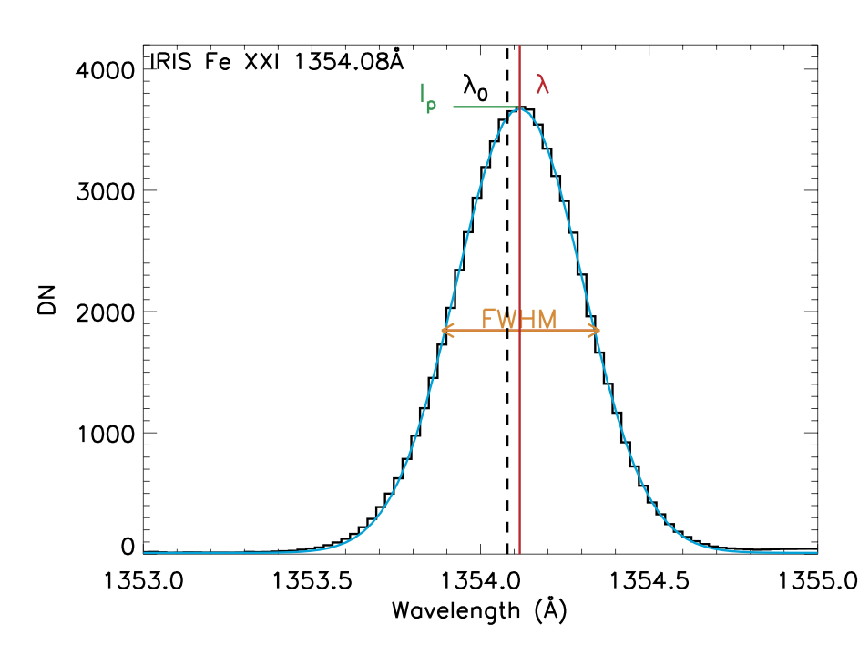
Figure 4.1: Example of Gaussian fit of the Fe XXI 1354.08 Å line observed by IRIS using the routine gaussfit.pro.

4.1.1. Single-Gaussian fitting¶

There are several IDL routines which can perform a single Gaussian fit of a line, some of them are listed below. In the following, wvl and sp indicate the wavelength array and spectrum of the IRIS line respectively.

function gaussfit

Purpose: Computes a non-linear least-squares fit to a function f (x) with from three to six unknown parameters.

Usage:

yfit = gaussfit (wvl, sp, A, NTERMS=nterms [+keywords])

Parameters

A: is the variable that contains the coefficients of the fit
NTERMS is an integer value between 3 and 6 used to specify the function for the fit.

For example, if NTERMS=5,

\[f (x) = A \left[ 0 \right] \cdot exp^{\frac{-z^2}{2}}+A\left[ 3 \right] + A\left[ 4 \right] \cdot X\]

where \(A \left[ 0 \right]\) is the peak value, \(z = \frac{x-A[1]}{A[2]}\) with \(A \left[ 1 \right]\) being the peak centroid and \(A \left[ 2 \right]\) the gaussian \(\sigma\). Using the results of the fit, the FWHM and totally intensity of the line can be calculated as follows:

\[FWHM = 2\sqrt{2ln2} \cdot A \left[ 2 \right]\]

\[I_\textrm{TOT} = \sqrt{2\pi} \cdot A \left[ 0 \right] \cdot A \left[2 \right]\]

See the IDL documentation http://www.harrisgeospatial.com/docs/GAUSSFIT.html for a list of all the keywords and more details on this routine.

function mpfitpeak

Similar to gaussfit.pro but can be used also to fit a Lorentzian or Moffet function.

Usage:

yfit = mpfitpeak (wvl, sp, A, NTERMS=nterms [+keywords])

See the IDL documentation http://www.harrisgeospatial.com/docs/mpfitpeak.html for more details on the mpfitpeak.pro routine.

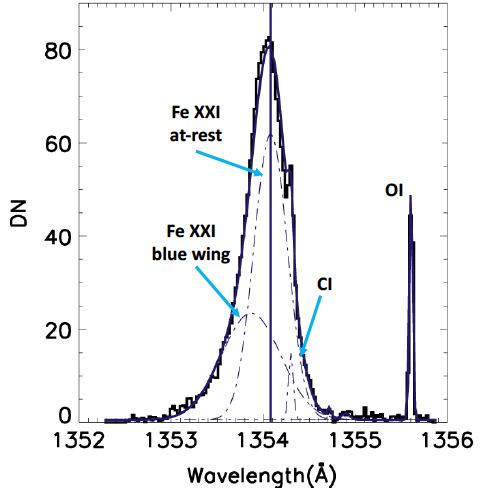
Figure 4.2: Example of a multi-Gaussian fit for the IRIS OI 1355.6 spectral window. The Fe XXI 1354.08 Å, C I 1354.30 Å and O I 1355.60 Å lines are indicated by the respective labels. The Fe XXI line has been fitted with two Gaussian components (indicated by the dotted blue lines): one at-rest dominant component and one fainter component on the blue wing of the line. In addition, the C I line is partially blended on the red wing of the Fe XXI line. Adapted from: Polito et al. 2015, ApJ, 803, 84.

4.1.2. Multi-gaussian fitting¶

For a double-(or multi-) Gaussian fit (see Figure 4.2 ), the following routines may be used:

function cfit and xcfit

Purpose: Given a structure describing the set of components to be fitted, finds the best fit of the sum of components to the supplied data

Usage:

yfit = cfit(wvl, sp, A, fit [,SIGMAA] [+keywords])

Parameters:

A : Array of parameter values before/after fit. If defined on entry, then these values are used as initial values for the fit, unless the reset keyword is set.
fit : Fit structure containing one tag for each component in the fit.
sigmaa : Errors for each of the parameter values included in A.

xcfit.pro is the widget-based version of cfit.pro which allows the interactive design of the fit structure. See https://hesperia.gsfc.nasa.gov/ssw/gen/idl/fitting/cfit.pro, https://hesperia.gsfc.nasa.gov/ssw/gen/idl/fitting/xcfit.pro and http://darts.jaxa.jp/pub/solar/sswdb/soho/cds/lrg_data/info/swnote/cds_swnote_47.pdf.

4.1.3. 2D automatic fitting¶

To perform an automatic fit over the 2D X- and Y- spatial arrays in a IRIS raster for a particular spectral line, one can either use the routines described above and repeat the fit for each of the pixels or use some dedicated routines to handle 2D data arrays, as described below.

pro iris_auto_fit

Purpose: automatically fits single or multiple Gaussians to two-dimensional spatial arrays.

Usage:
iris_auto_fit, windata, fitdata, /perpixel [+keyword]
Parameters:

windata: the window data cube

fitdata: a structure containing the fit (see below)

To extract information from the FITDATA structure, one can use:

IDL> intensity = eis_get_fitdata(fitdata, /int)
IDL> velocity = eis_get_fitdata(fitdata, /vel)
IDL> width = eis_get_fitdata(fitdata, /wid).

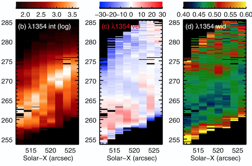
iris_auto_fit is adapted from eis_auto_fit, which was originally written by Dr Peter Young for the analysis of Hinode/EIS data. More information can be found at: http://www.pyoung.org/quick_guides/iris_auto_fit.html. An example of automatic fit of the IRIS Fe XXI line profile is shown in Figure 4.3

Figure 4.3 Intensity (left panel, in logarithmic scale), Doppler shift (middle panel) and width (right panel) of the IRIS Fe XXI line obtained by using the automatic fitting routine iris_win_fit.pro applied to IRIS data. Adapted from Figure 12 of `Young et al 2015, ApJ, 799, 218.

4.2. Wavelength calibration¶

When measuring Doppler shifts in spectral lines, it is important to perform an accurate absolute calibration of the wavelength array.

Note

The wavelength calibration is automatically performed in IRIS level 2 data. However, this should be always checked manually using the centroid positions of strong neutral lines, which are not supposed to vary significantly over time (within an uncertainty of 5–10 km s ^-1). Suitable lines for performing the wavelength calibration are the O I 1335.60 Å line for the FUVS detector, the S I 1401.515 Å line (when strong enough) for the FUVL detector and the Ni I 2799.474 Å line in the NUV.

4.3. Radiometric calibration¶

The intensities of IRIS spectral lines should always be converted in physical units (e.g. from DN to erg cm ^-2 s ^-1 sr ^-1 or phot cm ^-2 s ^-1 arcsec ^-1) before comparing the intensities of different lines and/or using them as plasma diagnostics tools (see Sect. 5).

The calibration data is included in the IRIS solarsoft branch, and Sect. 6.2 of ITN 26, Calibration of IRIS observation shows in details how to perform the radiometric calibration of IRIS lines. In addition, one might use the IDL routine iris_calib.pro written by Dr. Peter Young.

pro iris_calib

Purpose: converts an IRIS DN value to erg cm ^-2 s ^-1 sr ^-1

Usage:
iris_calib, int, wavelength, date, texp=texp, [+keywords]

Parameters

int: the total intensity of the line in DN

wavelength : the wavelength of the line in Angstrom

date: the date of the observation in a standard SSW format.

texp: the exposure time in seconds. If not specified, then 1 second is assumed.

Note

The exposure time texp can be different for each exposure in the same sequence, when the Automatic Exposure Control (AEC) is switched on. See the note in Sect. 6.2 of ITN 26, Calibration of IRIS observation for more information.