1. Diagnostics of Photospheric Lines in the Wings of Mg II h & k
1.1. Photospheric Diagnostics
This tutorial will guide you through the calculation of the photospheric diagnostics from a list of photospheric spectral lines observed in the IRIS NUV spectral windows. The majority of the lines is found in the Mg II k 2796 spectral window. See Table Table 1.1 below (from Pereira et al. 2013) with a list of rest wavelengths, formation heights and uncertainties for several photospheric lines.
| Species | Wavelength [Å] | Formation Height [Mm] | Uncertainty [Mm] |
|---|---|---|---|
| Cr II | 2787.295 | 0.17 | 0.02 |
| C I | 2810.584 | 0.17 | 0.03 |
| Ni I | 2815.179 | 0.17 | 0.03 |
| Ni I | 2816.010 | 0.17 | 0.03 |
| Ti II | 2785.465 | 0.22 | 0.03 |
| Cr II | 2786.514 | 0.21 | 0.03 |
| Fe I | 2809.154 | 0.28 | 0.05 |
| Fe I | 2792.327 | 0.38 | 0.03 |
| Fe I | 2806.634 | 0.38 | 0.03 |
| Fe I | 2806.897 | 0.42 | 0.03 |
| Fe I | 2793.223 | 0.50 | 0.04 |
| Cr II | 2801.584 | 0.58 | 0.03 |
| Fe I | 2805.690 | 0.58 | 0.03 |
| Ni I | 2805.904 | 0.58 | 0.06 |
| Fe I | 2798.600 | 0.64 | 0.06 |
| Ni I | 2799.474 | 0.68 | 0.07 |
| Fe I | 2805.346 | 0.68 | 0.09 |
| Mn I | 2795.641 | 0.74 | 0.09 |
| Fe I | 2799.972 | 0.76 | 0.07 |
| Fe I | 2814.116 | 0.76 | 0.11 |
| Fe I | 2788.927 | 0.88 | 0.11 |
| Mn I | 2799.094 | 0.84 | 0.11 |
| Mn I | 2801.907 | 0.83 | 0.10 |
Multi-line velocity diagnostics are a powerful tool for tracing the vertical velocity structure (e.g. Lites et al. 1993; Beck et al. 2009; Felipe et al. 2010). Generally speaking, the lower the photospheric height, the more reliable the velocity estimates. This is related to the increased corrugation of formation heights as the lines get stronger (Pereira et al. 2013).
Many lines listed above are “blended”, i.e. they are found in close proximity to strong chromospheric lines (i.e. the Mg II k and h lines, Mg II triplet line) as well as near other photospheric lines of Table 1. Blending renders lines to have profiles that are hard (or even impossible) to fit with a Gaussian profile. Through experimentation we have found the following lines to be almost blend free (Table Table 1.2).
| Species | Wavelength [Å] | Formation Height [Mm] | Uncertainty [Mm] |
|---|---|---|---|
| Ni I | 2815.179 | 0.17 | 0.03 |
| Fe I | 2792.327 | 0.38 | 0.03 |
| Fe I | 2793.223 | 0.50 | 0.04 |
| Cr II | 2801.584 | 0.58 | 0.03 |
| Fe I | 2805.690 | 0.58 | 0.03 |
| Ni I | 2805.904 | 0.58 | 0.06 |
| Ni I | 2799.474 | 0.68 | 0.07 |
| Fe I | 2805.346 | 0.68 | 0.09 |
| Fe I | 2799.972 | 0.76 | 0.07 |
| Fe I | 2814.116 | 0.76 | 0.11 |
| Mn I | 2801.907 | 0.83 | 0.10 |
Start by downloading an IRIS dataset from 2014 March 29: follow this link and download the slit-jaw files and the raster file (about 6 Gb in total). Download them to a directory of your choice (here we’ll call it ~/iris_data/). Unzip all the files, e.g. on a UNIX system:
% gunzip *fits.gz
% tar zxvf *.tar.gz
This sparse 8-point raster series is comprised of 179 rasters, totaling 4 hours of observations. During this long period of time, the orbital velocity and thermal drifts went through significant changes. For accurate Doppler calibration of these photospheric lines, these effects must be taken into consideration.
In this tutorial we will use Interactive Data Language (IDL), so let’s begin by loading the data using the IDL object interface:
% sswidl
(...)
ff=iris_files('*l2*_r0*.fits')
irisobj = iris_obj(ff[0])
As we mentioned above, we need to correct for orbital velocity and thermal drifts (to be used later; note that it may take a while depending on the size of the data series):
iris_orbitvar_corr_l2s,ff[*], dw_orb_fuv, dw_orb_nuv, date_obs
dw_orb_nuv=reform(dw_orb_nuv, n_slit, n_elements(dw_orb_nuv)/n_slit)
date_obs=reform(date_obs, n_slit, n_elements(date_obs)/n_slit)
Also, load the SJI images for reference:
fsji=findfile('iris_l2_20140329_140938_3860258481_SJI_1400_t000.fits')
read_iris_l2, fsji, indsji, SJI
Let us see the spectral windows that are saved in this raster:
irisobj->show_lines

;The above command should return the following windows for this data series:
;Spectral regions(windows)
;0   1335.71   C II 1336
;1   1343.31   1343
;2   1349.43   Fe XII 1349
;3   1355.60   O I 1356
;4   1402.77   Si IV 1403
;5   2832.74   2832
;6   2826.59   2826
;7   2814.46   2814
;8   2796.20   Mg II k 2796
Now get the centering information and timing information for each slit position for the entire time-series:
n_win=irisobj -> getnwin() ;get number of spectral windows present in OBS ID

;get coordinates and time for each slit
xpos=irisobj->getxpos()
ypos=irisobj->getypos()
xtime=irisobj->ti2utc()
timei=xtime
n_slit=n_elements(xtime[*,0])
Also, get exposure time in spectral windows – needed later:
exptimiris=fltarr(n_elements(xpos), n_win)
for jj=0, n_win-1 do exptimiris[*,jj]=irisobj->getexp(iwin=jj)
We will focus on window 8, since it contains the majority of the lines:
iwin=8
Let’s see where the slits positions are located on a slit-jaw image. First, get the following info:
;header
head = irisobj->gethdr(fix(iwin))

;Store into variables the spatial spacing and the resolution across the slit::
xincrement=sxpar(head, 'CDELT3') ;sparse raster density
dy=sxpar(head, 'CDELT2')
dlambda=sxpar(head, 'CDELT1')
For this example we will focus on the first slit of the first raster:
m=0 ;raster number
slit=0 ;slit position of raster
yheight=400 ;pixel location (or height) along slit
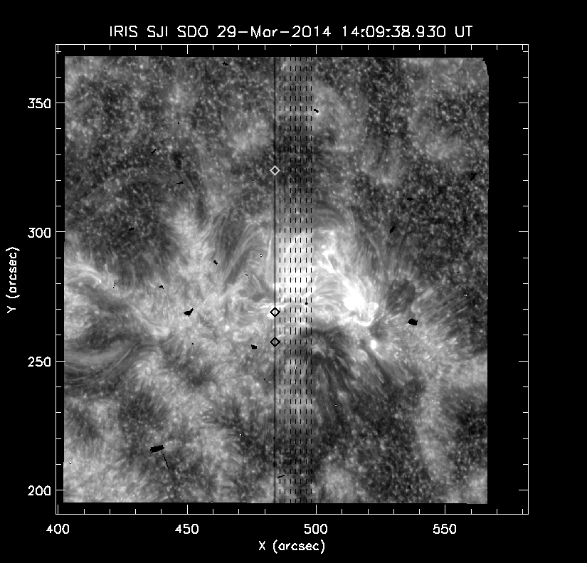
;Plot the slit positions of the first raster onto the first 1400 SJI image::
index2map, indsji[0], sji[*,*,0], mapsji
plot_map, mapsji, /log, charsiz=1.8, charthick=2 , dmin=5, dmax=1200
oplot, xpos[slit]+fltarr(n_elements(ypos[*])), ypos[*], col=0
for ii=0, n_slit-1 do oplot,(xpos[ii]#(1.+fltarr(n_elements(ypos[*])))),((1.+fltarr(n_slit))#ypos[*])[ii,*], linesty=2, col=0
;So the position of the 400-th pixel along the first slit is at the location of the diamond symbol:
plots, xpos[slit], ypos[yheight], psym=4, col=0, symsize=2, thick=2
For the line fitting we will pick one line at this specific location of the first raster, the Fe I 2792.327, which forms at 0.38 Mm according to Table 2:
linewinassign=iwin ;i.e pick the spectral window from list above – Mg II
linecphot=2792.327 ;Rest wagelength (in A)
linecheight=0.38  ;Mm
linecheightuncert=0.03 ;Mm
namephot='Fe I 2792.3270'
Perform the following commands to extract the spectrum from the object we created earlier for the first raster:
wave = (irisobj->getlam(iwin)) ;<--- this contains the wavelength!!
spec = irisobj->getvar(iwin) ;<--- this contains the spectrum!!
nraster = irisobj->getinfo('NAXIS3', iwin) ;<---get number of raster columns
ss = size(spec)
nspec = ss[2] ;get number of y-pixels along slit

specc=fltarr(nraster, ss[2], ss[1]) ;ss[1] is the spectral dimension
for iii=0, nraster-1 do specc[iii,*,*]=transpose(irisobj->descale_array(spec[*,*,iii]), [1,0]) ;specc dimensions [x, y, lambda]

imm=(transpose(specc[*,*,*],[2,1,0]))[*,*,slit];after transp it is [y,lam,x]
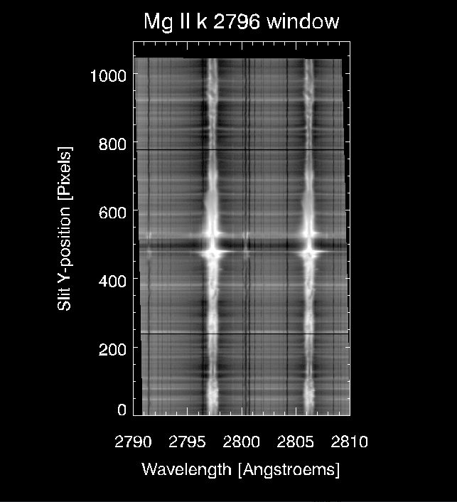
The variable imm now contains an image of the spectrum in the Mg II 2796 window along the slit y, of dimensions [y,lambda,x], where x is the slit number (from 0 to 7 in this observation; slit=0 as we chose in previous step, thus this corresponds to the spectrum of the first slit). To visualize it:
plot_image, alog10(imm>0), min=1, max=3, xsty=1+4, title='Mg II k 2796 window', ytitle='Slit Y-position [Pixels]'
axis, xaxis=0, xrange=minmax(wave), /save, xtitle='Wavelength [Angstroems]'
axis, xaxis=1, xrange=minmax(wave), /save, xtickformat='(A1)'
In this spectral window the photospheric lines are seen as vertical absorption lines against the NUV continuum, amidst the Mg II k and h lines and the triplet lines which go into emission at certain locations across the slit. The two horizontal dark lines are due to the fiducial points which block the light in the spectrograph’s slit.
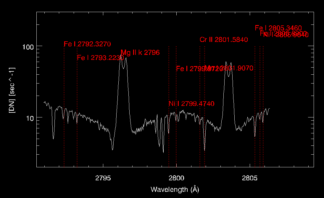
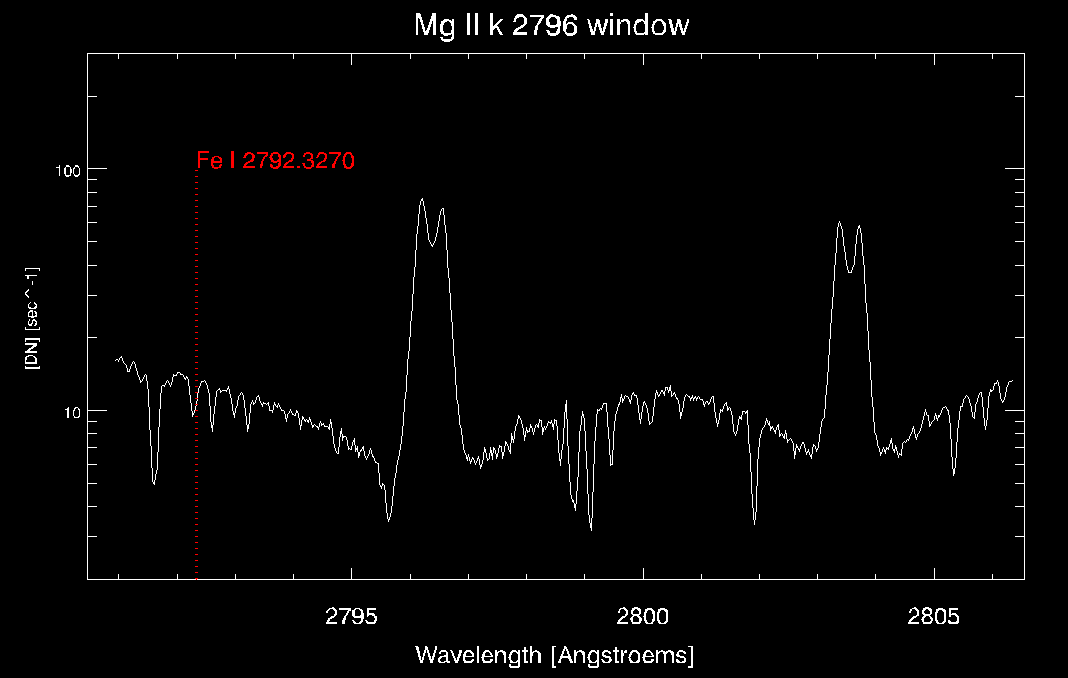
Let’s now plot the spectrum at the 400 pixel height and show where the spectral line is in the spectral window:
xtitle='Wavelength [Angstroems]'
ytitle='[DN] [sec^-1] '
title= 'Mg II k 2796 window '

Ymin=2 & ymax=300
erase
plot, imm[*,yheight]/exptimiris[slit, iwin, m], xtickformat="(A1)", ystyle=1+4, xstyle=1+4, /noerase,/ylog, yrange=[ymin, ymax], ytitle=ytitle,/nodata, xtitle=xtitle, title=title

axis, yaxis=0, ystyle=1,  yrange=[ymin, ymax],ytitle=ytitle, charsiz=2, /ylog,/sav
axis, xaxis=0, xstyle=1,  xtitle=xtitle, xrange=minmax(wave),/save, xticks=0, xminor=0, xticklen=0
axis, xaxis=1, xstyle=1,  xtickformat="(A1)", xrange=minmax(wave), xticks=0, xminor=0, xticklen=0
axis, yaxis=1, ystyle=1,  yrange=[ymin, ymax],ytickformat="(A1)", /ylog, /save
oplot, wave,imm[*,yheight]/replicate(exptimiris[slit, iwin, m], n_elements(imm[*,yheight]))

loadct, 13, /sil
oplot, linecphot+fltarr(ymax/3),indgen(ymax/2),linesty=1, color=255, thick=3
xyouts, linecphot,ymax/3,namephot, orient=0,align=0
loadct, 0, /sil
Now that we have identified the line we can proceed with line fitting; we will do that in a small spectral sub-window to isolate the line from nearby lines. Here, we chose a window size of 7 pixels.
winphot=7
indwvlphot=fltarr(n_elements(linecphot))
indwvlphot= (where(abs(wave-linecphot) eq min(abs(wave-linecphot))))[0]

;Before fitting, remove the orbital and thermal drifts from the wavelength array::

xdat=(wave)[indwvlphot+indgen(winphot)-round(winphot/2.)+1]+dw_orb_nuv[slit,m] ;remove thermal & orbital drift from wavelength array
ydat=double(imm[indwvlphot+indgen(winphot)-round(winphot/2),yheight])
Here we need to introduce a refinement stage for the sub-window centering. The photospheric lines typically span 4-5 spectral pixels with the IRIS NUV spectral resolution. However, neighboring lines may go into strong emission or absorption may have an impact in the intensity of the line wings for the line we are interested to perform a fit. In addition, a narrow (to account for the aforementioned issue) but fixed in size spectral window may cause problems when the photospheric line is strongly blue/redshifted, since it may not be completely sampled and/or the intensity at the wing locations would be underestimated, giving the impression of an asymmetric profile. For this purpose, we need to find the local minimum of the photospheric line profile and shift the spectral window to center the line as appropriate.
The final wavelength (xdata) and intensity (ydata) arrays to perform gaussian fitting:
temp =  where(smooth(ydat,2) eq min(smooth(ydat,2)))

if temp[0] ne -1 then begin $
xdata=(wave)[indwvlphot+indgen(winphot)-round(winphot/2.)+1+temp[0]-round(winphot/2)] &$
ydata=double(imm[indwvlphot+indgen(winphot)-round(winphot/2)+temp[0]-round(winphot/2),yheight]) &$
endif
We will be using a standard least-squares minimization fit routine called MPFITFUN, available in SSW/IDL distribution. We will have to provide constraints and initial guesses as follows:
xdatacen_estim=double(mean(xdata))

; Initial guess (amp, cent, width, background)
p0 =[-(max(ydata)-min(ydata)), xdatacen_estim, 0.035d, max(ydata)]
parinfo = replicate({value:0.D, fixed:0, limited:[0,0], limits:[0.D,0]}, n_elements(p0))
;now fix/constrain parameters
parinfo[*].value = [p0[0], p0[1], p0[2], p0[3]]
We can also provide an error array for the measurements – i.e. 1-sigma uncertainties:
poisnoise=18D ;photons/DN poisson noise from Pontieu et al 2014
readoutnoise=1.2D ;DN
err=sqrt((sqrt(ydata*poisnoise)/poisnoise)^2.+readoutnoise^2)
sy=1D/err^2. ;1/sigma^2
Create a gaussian function for MPFITFUN as an idl file called fit_funct.pro:
function fit_funct, x, a
   ; Evaluate the Gaussian parameters produced by mpfit
   ; x: input x array
   ; a: fit parmeters from mpfitpeak

   u = (x - a[1])/a[2]
   y = a[3] + a[0]*exp(-0.5*u^2)

   return, y
end
Now we can call that function through MPFITFUN and after providing the error estimates and constraints for the fit, we can obtain the best estimate for the gaussian fit coefficients and also the chi-square value (for this case it is 0.88):
coeff=MPFITFUN('fit_funct', xdata,ydata, err, /nan, parinfo=parinfo,/quiet)

chisq=total((ydata-fit_funct(xdata, coeff))^2*abs(sy))/(n_elements(ydata)-n_elements(coeff))
To see the result of the gaussian fit:
wln=interpol(xdata, winphot*5)
yfit=coeff[0]*exp(-0.5*((wln-coeff[1])/coeff[2])^2.)+coeff[3]

plot, wln, yfit, title=namephot, xtitle=xtitle, ytitle=ytitle
loadct, 13, /sil
oplot, wln, yfit, col=255
loadct, 0, /sil
oplot, xdata, ydata, psym=4
xyouts, mean(wln)-0.02, mean(yfit), string(chisq, FORMAT='(F5.2)'), col=100
xyouts, mean(wln)-0.04, mean(yfit)-30, string(linecheight, form='(f5.2)')+' Mm', col=150
oplot, replicate(linecphot,2), !y.crange, lines=1
oplot, replicate(coeff[1],2), !y.crange, lines=2
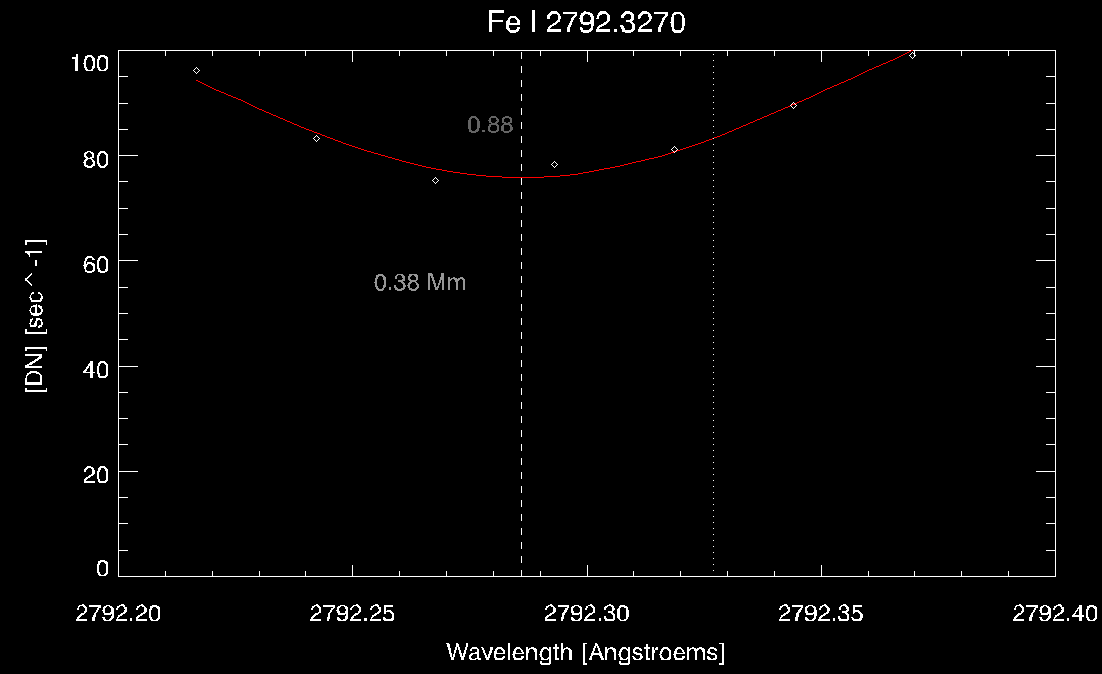
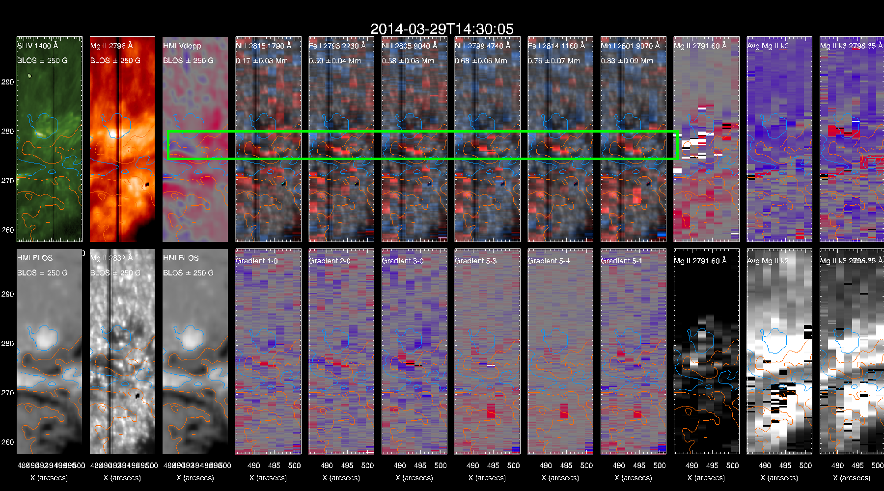
The dashed line shows the line center from the fit and the grey dotted line shows the rest wavelength for the Fe I line. This case shows a clear blueshift. If one performs the above exercise for all slit positions and for a range of y-positions along the slits we can obtain maps for the doppler velocities, intensities and line widths. Here’s an example where we show the doppler maps for selected photospheric lines and the doppler gradients for a combination of them along with maps of 2796, 2832 IRIS SJI and a magnetogram & photospheric Doppler from SDO/HMI for context.
1.2. Photospheric Temperature Diagnostics from the NUV Continuum
| Region | λi [nm] | λf [nm] | z [Mm] | Group |
|---|---|---|---|---|
| Mg II k far blue wing | 278.814 | 278.834 | 0.15±0.02 | 1 |
| Mg II k blue wing | 279.510 | 279.533 | 0.42±0.03 | 3 |
| Bump between h & k | 280.034 | 280.051 | 0.28±0.02 | 2 |
| Mg II h blue wing | 280.260 | 280.283 | 0.42±0.03 | 3 |
| Mg II h far red wing | 281.028 | 281.047 | 0.15±0.02 | 1 |
Using the above table (from Pereira et al. 2013), one can obtain the photospheric temperature, assuming the source function is identical to the Planck function. The latter is a reasonable assumption which allows to derive the radiation temperature, Trad. Therefore, we could convert the mean intensity found in the wavelength ranges of Table 3 and extract the radiation temperature at those three different heights.