2. Diagnostics based on the C II lines at 133.5 nm
2.1. Introduction
The IRIS spectrograph observes the Sun in three passbands, in the near ultraviolet band (NUV) and in the far ultraviolet, from 1332 to 1358 Å (FUV 1), and from 1389 to 1407 Å (FUV 2). The strongest lines in the FUV1 spectral domain are the resonance lines of singly ionized carbon (CII) around 1335 Å. This multiplet consists of three lines: one centered at 1334.53 Å and one line at 1335.71 Å with a weak blend in its blue wing at 1335.66 Å. Therefore, in the observations we see only two lines. The C II resonance lines sample the solar atmosphere from the upper chromosphere up to the transition region.
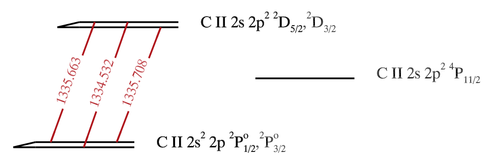
Fig. 2.1 C II lines at 1334-1336 Å between the \(2s\ 2p^{2}\ {}^{2}D\) and the \(2s^{2}\ 2p\ {}^{2}P^{0}\) terms. From Rathore & Carlsson (2015).
When calculated separately, C II multiplet lines reveal all three components that look like this:
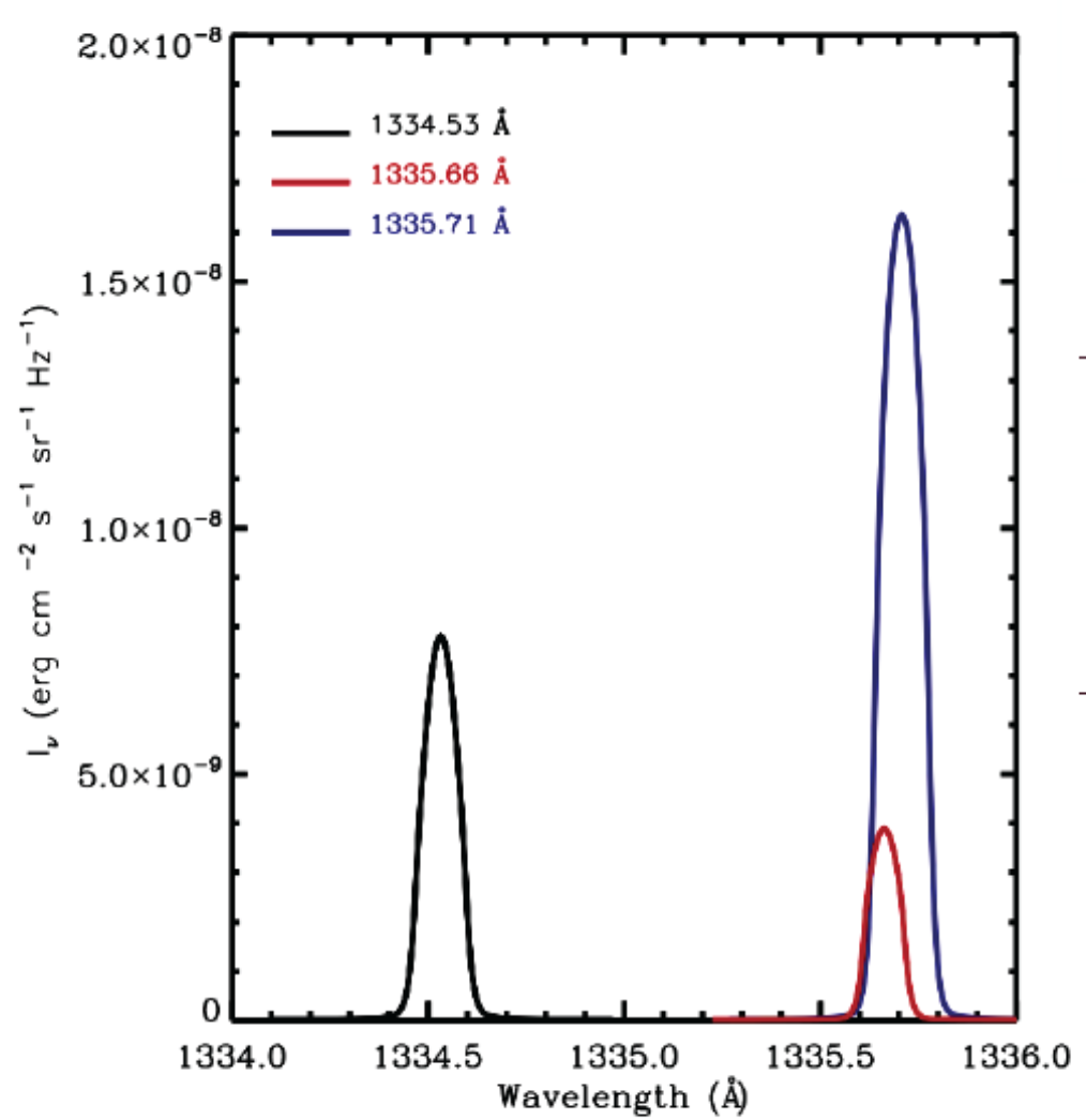
Fig. 2.2 The C II multiplet lines shown separately. The solid black, red and blue curves represent the C II 1334.53 Å, 1334.66 Å and 1334.71 Å lines, respectively. From Mats Carlsson’s tutorial for Optically Thick Line Formation and Interpretation of IRIS Observables: video and materials.
The formation of the C II lines is determined by the ionization balance, which is governed by the ionization and recombination rates between C II and C III (at high temperatures) and between C I and C II atoms (at low temperatures). The balance between C I and C II at the low temperature end depends on the atmosphere and is dominated by photoionization and radiative recombination. However, at the high temperature end, the ionization of CII is determined by collisional ionization and dielectronic recombination. When electron density dependence in dielectronic recombination is taken into account, compared to the default Chianti ionization balance (dashed line), there is less C II at the upper end of the temperature scale while a proper non-LTE treatment leads to more C II at the lower temperature end (solid line).
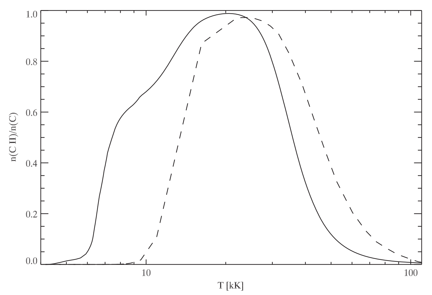
Fig. 2.3 C II ionization balance for the VAL3C model atmoshere (solid curve) as a function of temperature. The dashed line represents the default Chianti ionization balance. From Rathore & Carlsson (2015).
In order to decipher where are formed the C II lines, one can calculate the contribution function to the intensity at the line core. In the case of the C II 1334.53 Å line, it can be seen that the line core is formed between 10 and 40 kK. However, it is also possible for the line to be formed at lower temperatures. This depends on the transition region density. In a low density transition region, optical depth reaches unity at lower atmospheric layers where the temperature is lower as well. The contribution function to intensity also gives us information about the formation height of the line core, which is within the range between 2 and 4 Mm for this particular line. The total intensity mostly comes from the core formation region but there is also a broad tail of the contribution function going all the way down to the formation region of the continuum (which is, on average, around a height of 0.8 Mm).
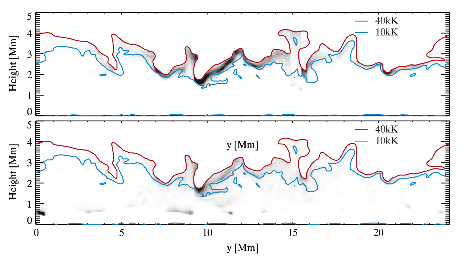
Fig. 2.4 Contribution function to intensity at the C II 1334.53 Å line core (upper panel) and to total intensity integrated over the line (lower panel). The model atmosphere is obtained with the Bifrost ( Gudiksen et al. 2011 ). Image taken from Rathore & Carlsson (2015).
The contribution functions to intensity and total intensity can also be given on a logarithmic column mass scale. In this way we can easily see that the transition region is less corrugated on a column mass scale than on a height scale. The other important conclusion that can be drawn is that the intensity, both at line core and for the integrated total intensity, is concentrated within a small column mass range. This is why the C II lines provide information about the solar chromosphere and the transition region. The same analysis holds for the C II 1335 Å line with the difference that this line is formed a little bit higher in the atmosphere.
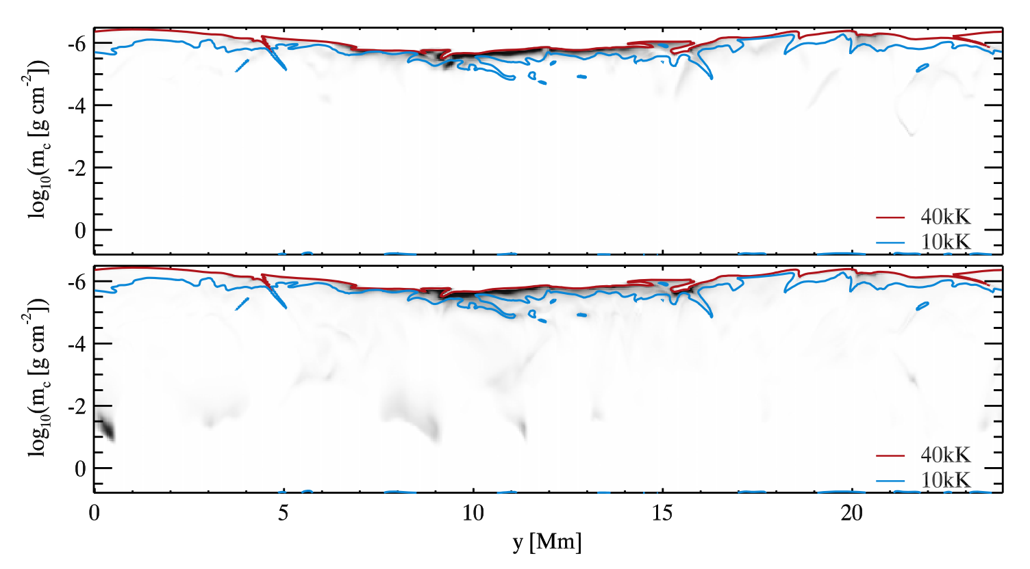
Fig. 2.5 Contribution function to intensity at the C II 1334.53 Å line core (upper panel) and to total intensity integrated over the line (lower panel) on a logarithmic column mass scale. From Rathore & Carlsson (2015).
Regarding the shapes of the C II line profiles, IRIS observations and 3D radiative magnetohydrodynamic simulations normally reveal one or two peaks, but in some cases the profiles can have three peaks or even be in absorption. The shapes of the C II lines are determined by the height variation of the source function and opacity. For example, single-peak profiles emerge due to monotonically increasing source function with height and up to the upper boundary where the line core has optical depth unity. On the other hand, double peak profiles are formed in the situations when the source function has a local maximum before it starts decreasing up until the height of optical depth unity in the line core. If source functions have multiple local maxima, we can observe the C II lines with more than two peaks. The presence of high velocity gradients can further complicate the shapes of the lines. Statistically, the number of single peak profiles in the CII 1334.53 Å line is larger than in the case of the line at 1335.71 Å. This can be explained by taking into account that the CII 1335.71 Å line is stronger, i.e., the optical depth unity is higher up in the atmosphere. Therefore, the probability that the line core is formed above the location where the source function has its local maximum (central reversal formation) is much higher.
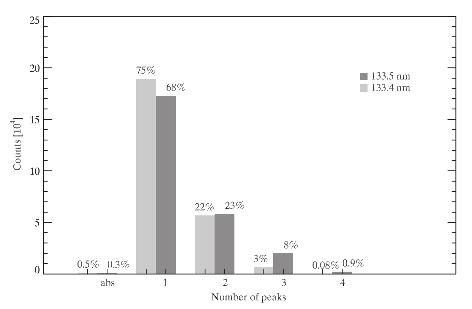
Fig. 2.6 The numebr of peaks has been derived from the simulation en024048_hion calculated with the 3D radiative magnetohydrodynamic (RMHD) code Bifrost. From Rathore et al. (2015a).
2.2. IRIS C II line diagnostics
The C II intensity filtergrams show a plethora of different features. Some of them closely resemble features visible in filtergrams taken in the Mg II h & k lines, while many others are similar to those seen in the transition region. This tells us that the C II lines are formed somewhere between the upper chromosphere and the transition region. This is the reason why the C II lines are good proxies for the atmospheric conditions in the upper chromosphere/lower transition region. It has been calculated that the ratio between the 1334.53 and 1335.71 Å components is always less than 1.8, which means they are optically thick lines.
2.2.1. Formation height
According to the Eddington-Barbier relation the disk center outgoing intensity is equal to the source function at optical depth unity, if the source function is a linear function of optical depth. However, this approximation can still be considered as good even when the source function is a non-linear function of temperature, as it is the case in the UV part of the solar spectrum. Therefore, considering the assumption that the Eddinggton-Barbier approximation is good for the optically thick C II 1335 Å lines, the correlation between the line core intensity and the source function at the optical depth unity should be a linear function (solid red line in figure below). As we can see, the correlation is indeed very good for the lower intensity values. However, the higher intensities show a small deviation from a linear function which is caused by a steep source function increase with height, which adds optically thin component to the intensity. Nevertheless, the Pearson correlation coefficient of 0.99 tells us that optical depth unity is a good approximation to the formation height as long as temperature gradient is not a steep, nonlinear function.
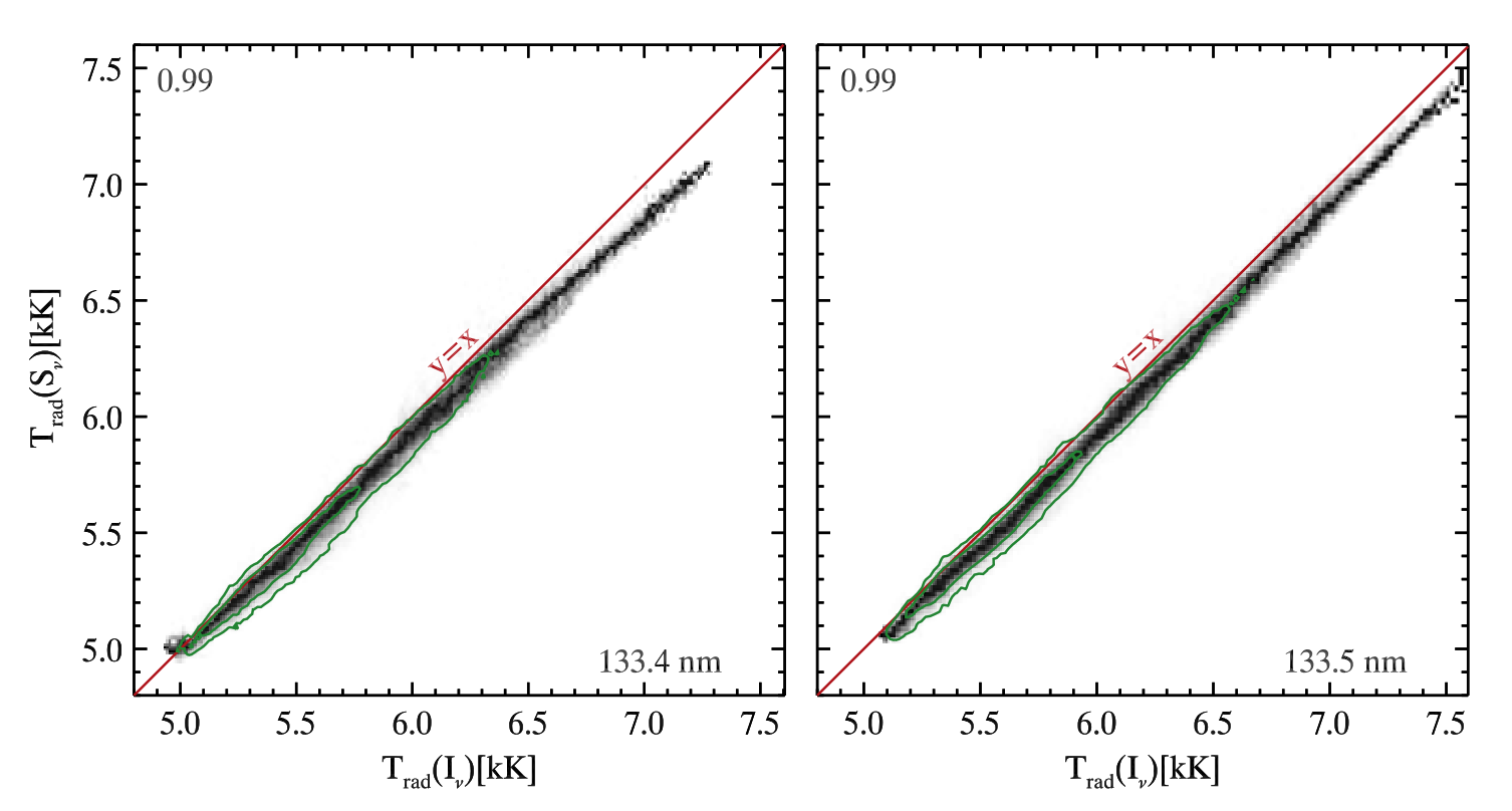
Fig. 2.7 The correlation between the line intensity at the line core and the source function at the optical depth unity. From Rathore et al. (2015a).
As we already mentioned above, the C II 133.4 nm and C II 133.5 nm lines are both formed just below the transition region height, i.e, the lowest height where the temperature is greater than 30 kK. Figure below shows relation between the transition region height and the formation height for the theoretical line cores. The difference in height is very small at the lower end of the scale, but increases as the transition region is formed higher in the atmosphere. However, there is a large scatter at the upper end of the scale, which is caused by false detection of the line cores. For example, due to large velocity gradient two peak profiles may have their peaks shifted so that they look like a single peak profiles and are identified as such by the core finding algorithm.
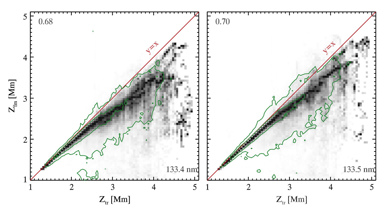
Fig. 2.8 PDF of formation height for the C II 133.4 nm line (left) and the C II 133.5 nm line (right) as a function of transition region height which is determined by the lowest height where the temperature exceeds 30 kK. The green contours enclose 50% and 90% of all points while the Pearson correlation coefficient is shown in the upper left corner. From Rathore et al. (2015a).
We can also take a look at histograms of the formation depth for single peak and non single peak profiles separately. These histograms show that single peak profiles are formed at smaller optical depths. Non single peak profiles are formed at higher optical depths due to the effects of steep nonlinear source functions.
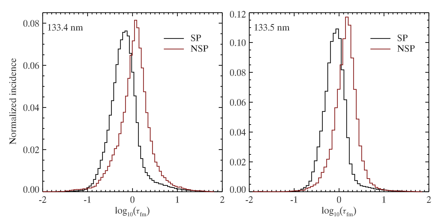
Fig. 2.9 Histograms of average formation height for single-peak (black) and non single peak (red) profiles, for the C II 133.4 nm and C II 133.5 nm lines. From Rathore et al. (2015a).
2.2.2. Intensity as temperature diagnostic
According to Rathore et al. (2015a), the line core intensity can be related to the temperature due to coupling between the Planck function and the source function, although the correlation is weak. Using the Bifrost simulation en024048_hion, it turned out that the temperature at the formation height is by a factor of two larger than the radiation temperature of the line core intensity for both of the C II lines. This also indicates that the source function has decoupled from the Planck function at the formation height.
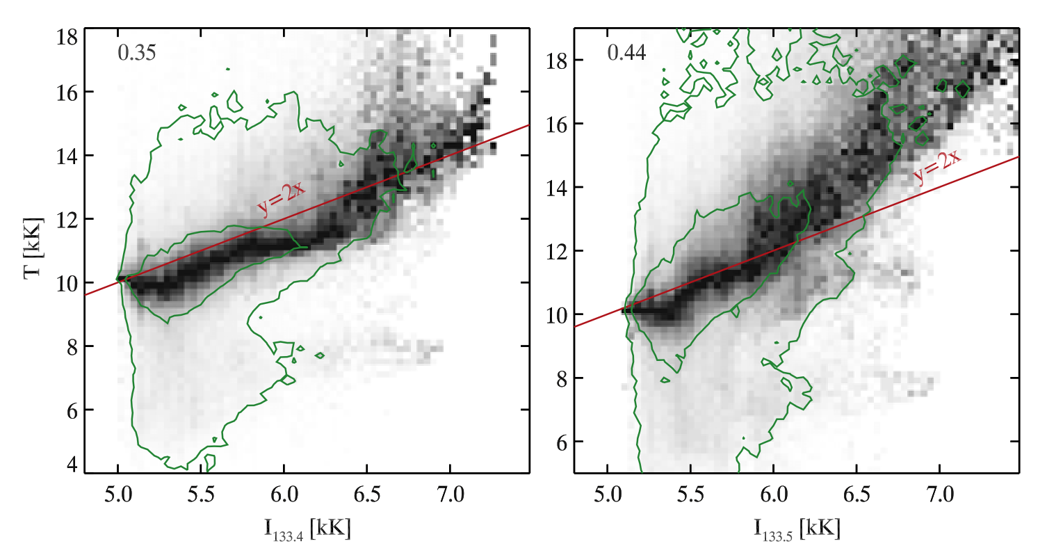
Fig. 2.10 PDF of the temperature at the formation height as a function of the radiation temperature derived from the C II 133.4 nm (left) and the C II 133.5 nm (right) line core intensities. The green contours enclose 50% and 90% of all points while the Pearson correlation coefficient is shown in the upper left corner. From Rathore et al. (2015a).
2.2.3. Line asymmetry
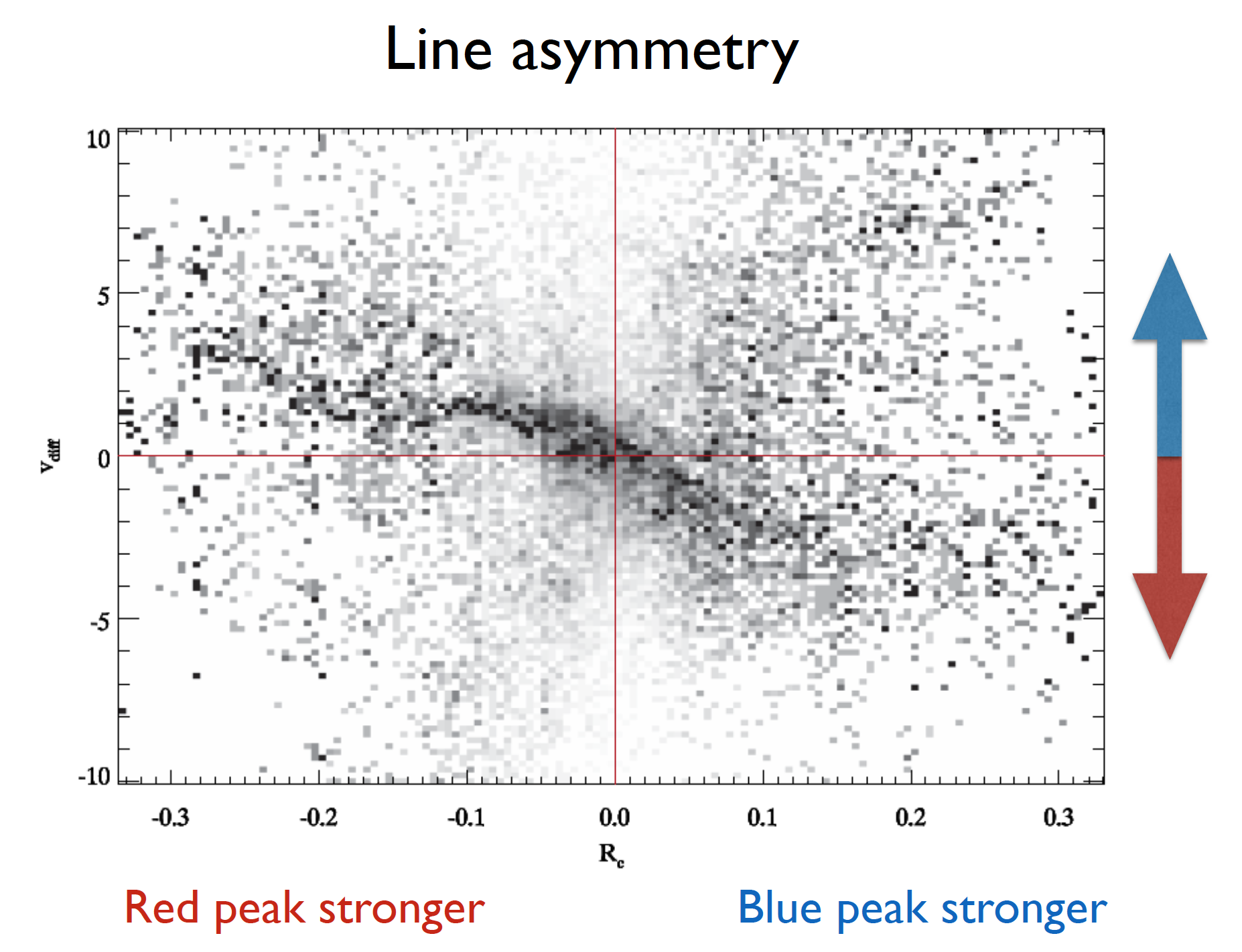
Leenaarts et al. (2013) demonstrated that double peak Mg II h and k profiles may exhibit an asymmetry where one peak is stronger than the other and this information can be used to infer the chromospheric velocities. Double peak lines can be explained by a presence of velocity gradient between the heights of formation of the line peaks and the core. Following the same approach as in Leenaarts et al. (2013), it can be seen that when blue peaks in the C II lines are stronger there is a downflow at the core formation height. Similarly, stronger red peak profiles are associated with upflows.
2.2.4. The line core Doppler shift
Doppler shift of single-Gaussian fit is well correlated with the line-of-sight velocity at the optical depth unity. However, there is some scattering in the relation which is the result of the identification algorithm. Taking into account that the C II 133.4 nm line is formed a few tenths of kilometers below the CII 133.5 nm line, the difference in Doppler shift between the two lines is most likely due to velocity gradient within their formation heights.
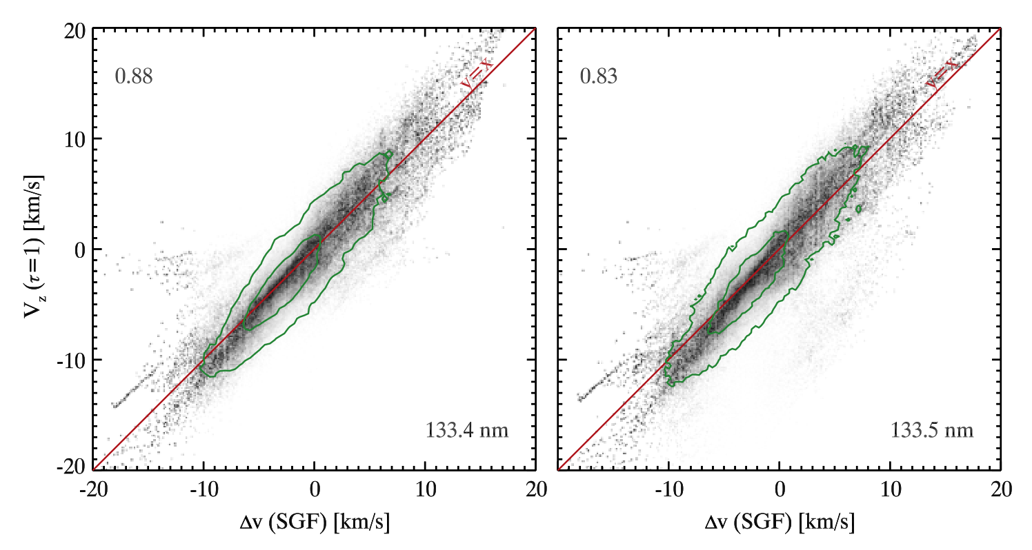
Fig. 2.12 Line-of-sight velocity at the optical depth unity as a function of Doppler shift of single-Gaussian fit for the C II 133.4 nm and C II 133.5 nm lines. From Rathore et al. (2015a).
2.2.5. Line width
The widths of the CII lines is well correlated with non-thermal velocities. It also depends on the temperature at the height of formation and so-called opacity broadening.
Note
Please note that the opacity broadening depends on the source function ratio between the formation heights of the continuum and the line core and is an additional broadening factor.
In this model, opacity broadening takes values in the range from 1.2 up to 4. It is small for single-peak profiles with a source function that rapidly rises into the transition region, and large when rapid increase of a source function occurs in the lower chromosphere and then either stay relatively constant or decrease. In other words, the source function with a peak in the lower chromosphere will produce steep emission flanks, i.e., a double peak intensity profile and therefore larger widths.
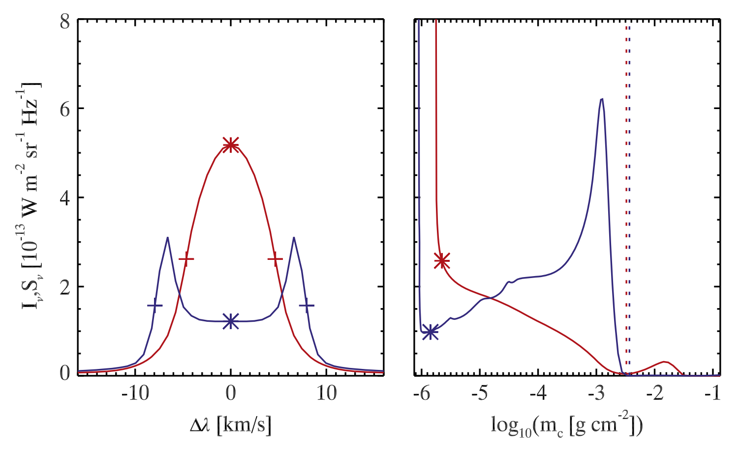
Fig. 2.13 Line intensity as a function of wavelength for two pixels from the Bifrost simulation (left) and their corresponding source functions as a function of logarithmic column mass (right). Asterisks indicate the intensities at the line core (left) and the corresponding heights for optical depth unity (right). Vertical dotted lines show the heights for optical depth unity in the continuum while plus signs denote the points corresponding to the FWHM widths. From Rathore & Carlsson (2015).
One can roughly characterize the widths of the C II lines using Gaussian fits. For this purpose, different parameters can be used, for example, the FWHM of the intensity profile (\(W_{FWHM}\)), the standard deviation of a single Gaussian fit (\(\sigma\)), the half width at \(\frac{1}{e}\) of the maximum intensity or \(\Delta V_{D}\). These parameters are defined for a Gaussian intensity profile as:
The upper left panel in the figure below shows that the FWHM is larger than \(1/e\) width (\(\Delta V_{D}\)) of a single Gaussian fit to the C II 1334.53 Å line profile, as most of the points lay above the red line (relation for a Gaussian profile). Or in other words, it means that the line profiles normally have a flatter top than a Gaussian profiles. This holds for the double-peak profiles as they are often much broader. However, in the lower right part of the same panel, there is a scattering which represents very asymmetric double-peak profiles where one peak is much weaker than the other. In this case \(W_{FWHM}\) is mainly determined by the width of the stronger peak, although the Gaussian fit is affected by the shape of the full profile. In the upper right panel, one can see the correlation between the measured widths of the C II 1334.53 Å profiles and the non-thermal velocity in the line-forming region (defined as 2 times the rms of the LOS velocities in the height formation range). It can be seen that the observed widths are well correlated with the non-thermal velocities in the atmosphere. The lower left panel shows a histogram of the non-thermal velocities with the maximum around 2 km/s. Finally, the lower right panel shows the opacity broadening factor as a function of \(\Delta V_{D}\). The broadening factor mostly takes values in the range from 1.2 up to 2, but could also be much higher and reach 4.
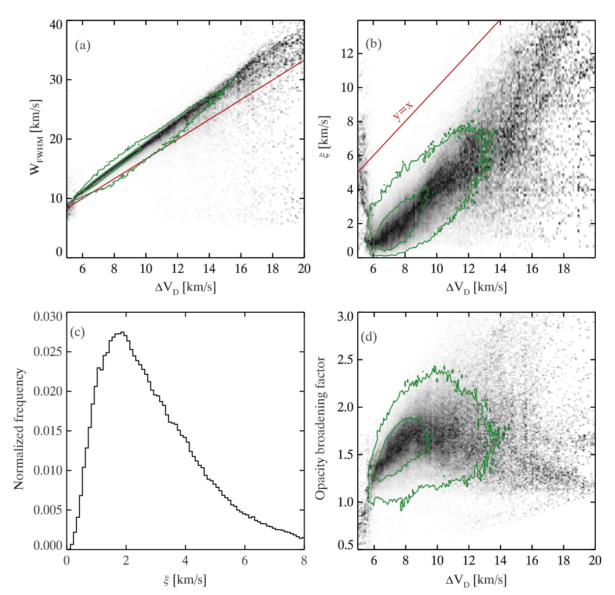
Fig. 2.14 Upper left: \(W_{FWHM}\) as a function of \(1/e\) width of a single Gaussian fit. Upper right: PDF of the non-thermal velocity ( \(\xi\) ) as a function of \(\Delta V_{D}\). Lower left: non-thermal velocities. Lower right: PDF of opacity broadening factor as function of \(\Delta V_{D}\). All displayed correlations are for the C II 1334.53 Å line. From Rathore et al. (2015a).
2.2.6. Comparison between the CII 133.5 nm, the MgII k and the Si IV 139.3 nm lines
Comparing the formation heights of the synthetic CII 1335 Å line, the Mg II k line and the Si IV 1393 Å line from the Bifrost simulation, it can be seen that the Si IV line is formed at a temperature around 80 kK under equilibrium conditions, while the the CII and Mg II k lines are formed lower in the atmosphere. It is interesting to note that sometimes the C II line can also be formed at a lower height compared to the Mg II k line, but this is not a common scenario. For the formation height of the CII and Mg II k lines is used the maximum \(\tau=1\) height and for Si IV the height of maximum emissivity as derived from CHIANTI.
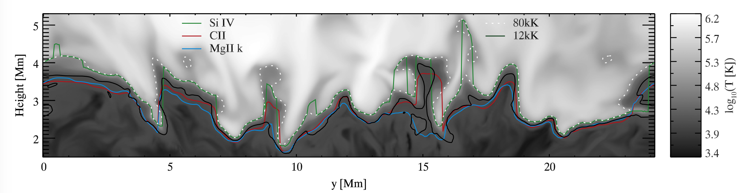
Fig. 2.15 Formation heights of the C II 1335 Å (red curve), the Mg II k (blue) and the Si IV 1393 Å (green) lines in Bifrost simulation. Temperature is given on a logarithmic scale with white dotted contour indicating 80 kK. 12 kK is marked by the black solid line. From Rathore et al. (2015a).
The formation heights of the C II 1335 Å and the Mg II k lines are shown in the figure below, but now considering the whole Bifrost simulation box. It is easily seen that the C II 1335 Å and Mg II k formation heights reveal very similar structures. However, the CII line is normally formed somewhat higher in the fibrils as can be seen in the central region of the simulation domain. There are also several small regions where formation height is significantly higher for the C II 1335 Å line. These regions are the result of cooler pockets of plasma that have enough density to put \(\tau=1\) there. On the other hand, the temperature is not low enough for Mg II k to reach optical depth unity there.
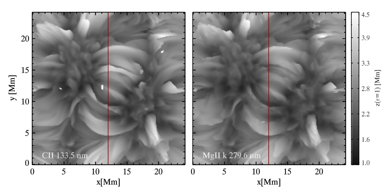
Fig. 2.16 Maximum height of optical depth unity over the line profile for the C II 1335 Å (left) and Mg II k (right) lines. From Rathore et al. (2015a).
2.2.7. Spatially averaged spectra
General characteristics of the C II line profiles in different regions on the Sun can be derived by averaging multiple intensity profiles. With this approach, it can be seen that the C II line intensity is normally weak inside QS internetwork regions, and increases in network, penumbra and umbra. The highest signal is detected in plage. All the profiles are shifted toward the red side, with respect to the rest wavelength of the line center. This redshift exhibits a very similar pattern to that of the intensity profiles, i.e., QS internetwork and network regions give rise to small redshifts, while in active regions the velocity shift is much larger. The other interesting characteristic of the C II line profiles is that in internetwork and network areas, the profiles show a slight central reversal, i.e., they are seen as double-peak profiles. On the other hand, the umbral, penumbral and plage profiles are normally single-peak in the 1334 Å line.
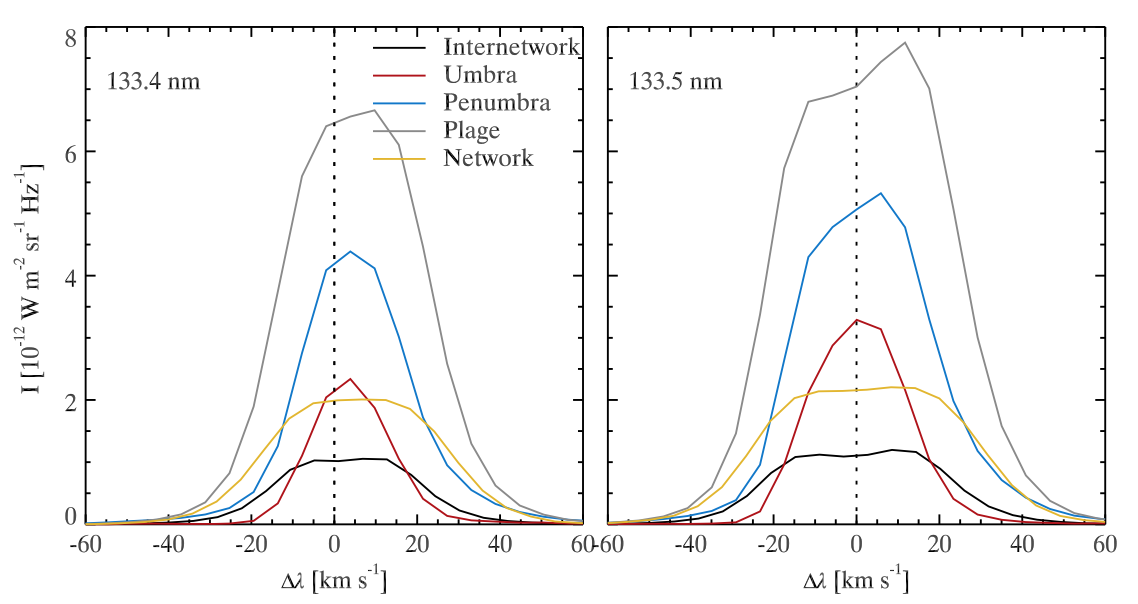
Fig. 2.17 Average intensity profiles of the C II 1334 and 1335 Å lines for different regions in the Sun. The rest wavelength of the line centers are marked with the vertical dotted lines. From Rathore et al. (2015b).
The C II lines are mostly single-peaked within active regions, while the lines formed in internetwork and network regions are dominated by single-peak profiles in the 1334 Å line, but not in the 1335 Å line. It is possible to detect triple-peak intensity profiles as well, but these are very rare.
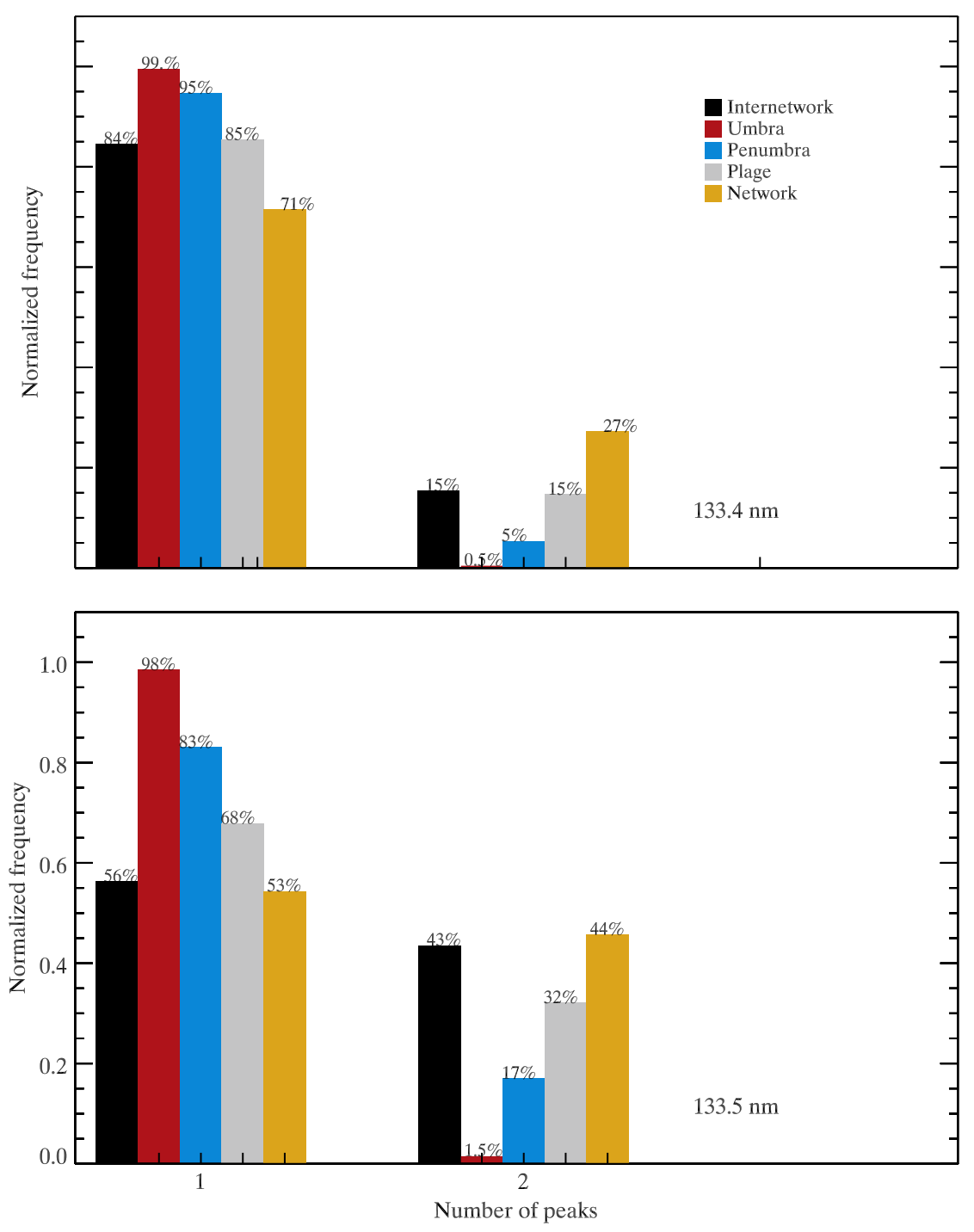
Fig. 2.18 Number of peaks for C II 1334 Å and 1335 Å lines in different regions. Different bar colors correspond to different regions on the Sun. From Rathore et al. (2015b).
If we now look at histograms of the ratio of the total line intensity for different solar regions, we can see that the C II lines are in all regions optically thick. The line ratio is almost always below 1.8. The lower ratios are found in the network regions (around 1.25), then in the internetwork and plage (~1.35), and finally the penumbral and umbral regions have the highest line ratio.
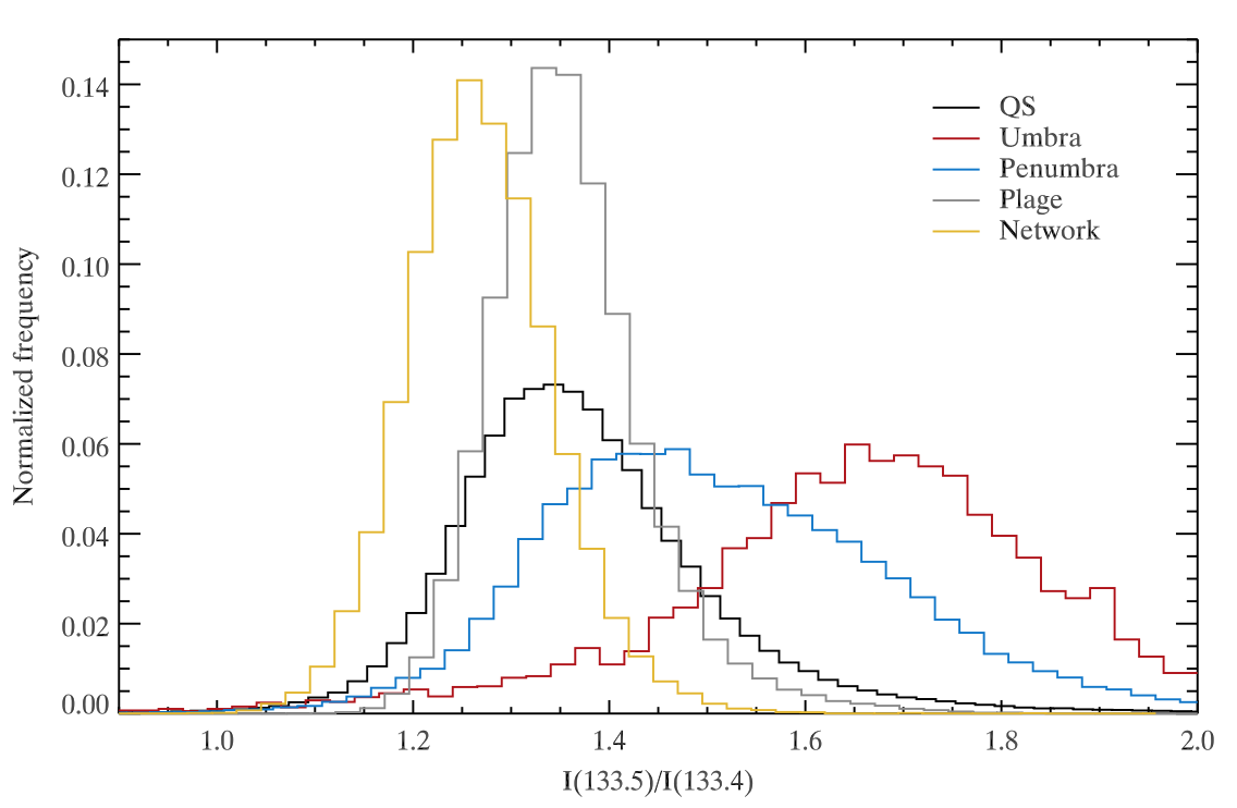
Fig. 2.19 Histograms of the ratio of total intensity between the 1335 Å and 1334 Å lines, for different regions. From Rathore et al. (2015b).
Rathore et al. (2015b) found an inverse correlation between the line widths and the line ratios. In general, the structures having larger line widths have smaller intensity ratios, and vice versa. Since double-peak profiles have a larger opacity broadening than single-peak profiles (i.e, a larger width), and have a lower intensity ratio, it is possible to draw important conclusions about physical conditions in different regions on the Sun. For example, the line ratio in the network is normally lower than in other regions, while the widths are largest. Therefore, a plausible explanation is that the increased width is to some extent the result of the larger opacity broadening for the profiles found within the network regions (double-peak profiles). If we now take into account that the internetwork is also dominated by double-peak profiles it looks like that thermal and non-thermal broadenings are larger in the network. There is also the possibility that the increased line broadening within the network is partially cause by motions of spicules or the chromospheric fibrils that are their disk conterparts. Furthermore, the plage and internetwork regions have similar widths, but since sigle-peak profiles are more common in plage (suggesting higher opacity broadening), it is expected that plage has larger non-thermal broadening than the internetwork.
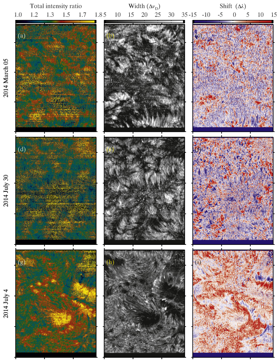
Fig. 2.20 Total intensity ratio of 1335 Å and 1334 Å (left column), line width of 1334 Å (middle column) and line shift of 1334 nm (right column). From Rathore et al. (2015b).
2.3. Diagnostic potential of the C I 1355.8 Å line
According to Lin et al. (2017) the C I 1355.8 Å emission line is dominated by a recombination cascade and is an optically thick line. Due to high correlation between the Doppler shift of the line and the vertical velocity in its line forming region (around 1.5 Mm), this line can be used along with optically thin O I 1355.6 Å line (formed slightly lower) to estimate the velocity difference between the line forming heights of the two lines. The ratio of the C I/O I line core intensity provides an additional information about the distance between the C I and the O I formation layers. This, together with the velocity difference, can further gives estimates on the velocity gradient in the middle chromosphere. The C I/O I total intensity line ratio is correlated with the inverse of the electron density.
2.4. References
Optically Thick Line Formation and Interpretation of IRIS Observables: video and materials
Gudiksen, B. V., Carlsson, M., Hansteen, V. H., et al. 2011, A&A, 531, A154
Leenaarts, J., Pereira, T. M. D., Carlsson, M., Uitenbroek, H., & De Pontieu, B. 2013, ApJ, 772, 90
Lin, H.-H., & Carlsson, M., Leenaarts, J. 2017, ApJ, 846, 40
Rathore, B., & Carlsson, M. 2015, ApJ, 811, 80
Rathore, B., & Carlsson, M., Leenaarts, J., & De Pontieu, B. 2015a, ApJ, 811, 81
Rathore, B., & Pereira, T.M.D., Carlsson, M., & De Pontieu, B. 2015b, ApJ, 814, 70