7. Tutorials
7.1. IRIS xfiles and CRISPEX
This tutorial will guide you step-by-step into some features of iris_xfiles and CRISPEX.
Start by downloading an IRIS dataset from 2013 December 26: follow this link and download the three slit-jaw files and the raster file (about 900 Mb in total). Download them to a directory of your choice (here we’ll call it ~/iris_data/). Unzip all the files, e.g. on a UNIX system:
% gunzip *fits.gz
% tar zxvf *.tar.gz
Start a solarsoft IDL session, and then launch iris_xfiles:
% sswidl
(...)
IDL> iris_xfiles
In the middle panel, next to Search Directory: press Change. Then navigate to the directory ~/data_temp/iris/20131226_171752_3840007146, press OK when this directory is selected. Notice that Search Pattern changed to free search. Make sure the time of these observations (2013 December 26, 17:17 UT) is contained in between the Start Time and Stop Time range, adjust if necessary.
Now press Start Search, and on the middle panel you will see a row with a summary of the observations, and a list of files on the bottom panel.
If you double click on the slit-jaw files, you can see a movie with Ximovie. In this case the observations are a 400-step raster of an active region. Because the slit-jaw images have been aligned to fixed coordinates on the Sun, the images are moving from left to right and black bars appear in the regions which are not exposed (the images are enlarged to fit the maximum extent of the observing sequence). With Ximovie you can adjust the display limits and also apply a gamma to the images.
If you double click on the raster file, an iris_xcontrol window will appear. This has a lot of information about the particular observing sequence, and displays some sample spectra and slit-jaw images. The middle spectral panel is split in the NUV (green-white) and FUV (red-white) spectrograms. You can also identify which spectral regions were observed. Clicking on either spectrogram will let you inspect individual spectrograms for all the steps in the sequence. You can also do the same with the SJI images.
Now we’ll use the profile moments tool. On the top left panel select the Mg II k 2796 line and under Line fit select Profile Moments. On the Moments Prep Tool window adjust the reference wavelength so that it matches the k3 core, and set the line start and stop so that it is about 5 pixels wide around k3. Set the continuum to be about 5 pixels wide on the right side of the plot, in a region with no absorption line, like the figure below.
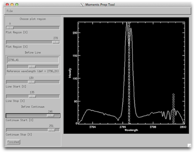
How the wavelength selection iris_xfiles moment tool should look like.
Press Finished. It will take a while to calculate the moments statistics in the region defined, and a new window opens. The result for intensity should look like the figure below.
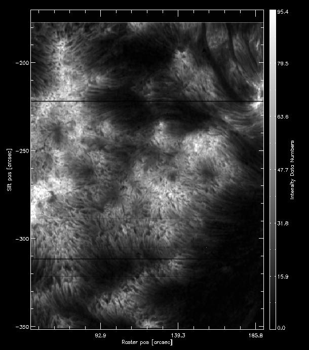
How the intensity from the k3 first moment should look like.
This looks very much like the Mg II k3 intensity, because we selected a very narrow window around it. On the bottom left side of the iris_xmap window you can also change Select data to show the first moment (centroid) velocity, but in this case this is not so reliable because we chose a small wavelength window.
Now to the same in Profile moments but select the k2v feature instead of k3. The result for intensity should look like the image below.
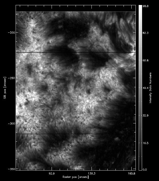
How the intensity from the k2v first moment should look like.
You can also experiment with the many other options of iris_xfiles as a quick way to explore the data.
Now we are going to create level 3 files from this set to use with CRISPEX. Go back to the IRIS_Xcontrol window of the raster file. Select the Si IV 1403 and Mg II k 2796 lines and press Generate level3 files. In the next dialog to not select anything and just press OK. We will use this level 3 file next with CRISPEX. Note that only one file will be created, as the time domain is missing.
Now start CRISPEX and use the name of the file you just created as an argument. Assuming you are in the same directory as the file, do:
IDL> crispex, 'iris_l3_20131226_171752_3840007146_t000_SiIV1403_MgIIk2796_im.fits'
It will take a while to start as CRISPEX calculates mean spectra and scaling factors. If everything went well you can start exploring the data. The main window will look black. This is because CRISPEX takes the first wavelength of the first line, in this case a wavelength in the continuum region of the Si IV 1403 line. The intensity here is mostly noise, so it appears as black. You can see the spectral windows in the other two windows: detailed spectrum and Spectral phi-slice.
Change the Main spectral position slider to around position 205. You can see on the spectra phi-slice that a vertical gray line moves. This indicates the current position in the spectrogram. Now you see more structure in the main image, but it is still a little dark. You can change the scaling in the Scaling tab: set the Histogram optimisation to 0.01 (this means that the scaling will be set from the 1% to 99% percentiles), or change the gamma to a lower value. On the Detailed spectrum window you still see only a vague outline of spectral lines. You can change this scaling in the Displays tab: set Lower y-value to -0.01 and the Upper y-value to 0.1. Now you should see the Mg II k line well, but the Si IV line is only visible for the brightest points.
When you move the mouse the windows update with the spectrum at the mouse pointer location. The Spectral phi-slice window shows a spectrogram with y being the position along a slit (the vertical white line that moves with the mouse cursor). If you click with the left button on a point it locks it. To unlock it you need to select the option Unlock from position on the middle of the main panel. Below it you can also see some properties of the current position: coordinates, wavelength being show, time, data values, etc.
You can change the parameters of the slit made to construct the Spectral phi-slice window. On the Spectral tab, middle part, there are controls named Slit controls. There you can adjust the angle and length of the slit, and see how the window changes.
7.2. Mg II Dopplergrams
In this tutorial we are going to produce a Dopplergram for the Mg II k line from an IRIS 400-step raster. The Dopplergram is obtained by subtracting the intensities at symmetrical velocity shifts from the line core (e.g. ±50 km/s). For this kind of analysis we need a consistent wavelength calibration for each step of the raster.
Start by downloading an IRIS dataset from 2014 July 8: follow this link and download the raster file (726 Mb). Download it to a directory of your choice. Untar it, e.g. on a UNIX system:
% tar zxvf iris_l2_20140708_114109_3824262996_raster.tar.gz
Feel free to examine these data in iris_xfiles. This very large dense raster took more than three hours to complete the 400 scans (30 s exposures), which means that the orbital velocity and thermal drifts were changed during the observations. This means that any precise wavelength calibration will need to correct for those shifts.
First lets start sswidl and load the data using the IDL object interface:
% sswidl
(...)
IDL> filename = 'iris_l2_20140708_114109_3824262996_raster_t000_r00000.fits'
IDL> d = iris_obj(filename)
Let us see the spectral windows that are saved in this raster:
IDL> d->show_lines
Spectral regions(windows)
0   1335.71   C II 1336
1   1349.43   Fe XII 1349
2   1355.60   O I 1356
3   1393.78   Si IV 1394
4   1402.77   Si IV 1403
5   2832.70   2832
6   2814.43   2814
7   2796.20   Mg II k 2796
Let us load the Mg II lines into memory:
IDL> wave = d->getlam(7)
IDL> data = d->getvar(7, /load)
We can see how the the spatially averaged spectrum looks like:
IDL> mspec = total(total(data, 2), 2)
IDL> plot, wave, mspec
IDL> plot, wave, mspec, xrange=[2794, 2799], /xst
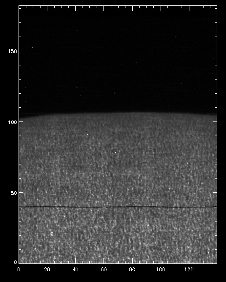
To better understand the orbital velocity problem let us look at how the line intensity varies for a strong Mn I line at around 280.2 nm, in between the Mg II k and h lines. For this dataset, the line core of this line falls around index 350. To plot it in the correct orientation we will make use of IDL’s transpose, and the procedure pih (available in the IRIS tree of solarsoft) to make the plot:
IDL> pih, transpose(reform(data[350,*,*])), min=0, max=200, scale=[0.35,0.1667]
The result should look like this:

Intensity at Mn I 280.2 nm line line when orbital velocity and thermal drifts are not accounted for.
You can see a regular bright-dark pattern along the x axis, and indication that its intensities are not taken at the same position in the line because of wavelength shifts.
To calculate the wavelength shifts from the orbital velocity and thermal drifts we do the following:
IDL> wavecorr = iris_prep_wavecorr_l2(filename)
This routine measures the wavelength position of 5 neutral lines (3 NUV, 2 FUV) whose rest wavelengths are reasonably well known, and saves the shifts (in Ångström) into the structure variable called wavecorr. The structure format is as follows:
IDL> help, wavecorr
** Structure <484f608>, 14 tags, length=3552144, data length=3552140, refs=1:
NOTE            STRING    'corrs[file, rasterstep, line] gives target_wave - measured_wave in angstroms'
FILES           STRING    'iris_l2_20140708_114109_3824262996_raster_t000_r00000.fits'
LNAME           STRING    Array[5]
WAVE0S          FLOAT     Array[5]
TIMES           STRING    Array[1, 400]
TAIS            DOUBLE    Array[1, 400]
NX              LONG               400
NY              LONG              1094
COORD           FLOAT     Array[1, 400, 1094, 2]
CORRS           DOUBLE    Array[1, 400, 5]
CHISQ           DOUBLE    Array[1, 400, 5]
CORR_TAI        DOUBLE    Array[400]
CORR_NUV        DOUBLE    Array[400]
CORR_FUV        DOUBLE    Array[400]
Note
A vector of level 2 fits raster files can also be passed to iris_prep_wavecorr_l2 instead of a single file; this example uses a single raster, so it has a single file, and as a result the leading dimension is 1 for the corrs, chisq, times and tais fields in the wavecorr structure.
The five spectral lines that have been measured are as follows:
IDL> for i = 0, 4 do print, wavecorr.lname[i], wavecorr.wave0s[i]
Ni I      2799.47
Mn I      2801.90
Fe I      2805.35
O I       1355.60
Fe II     1392.82
The wavelength shift in the i-th line in the j-th frame of the k-th input file is stored in wavecorr.corrs[k, j, i] . Averaged and smoothed corrections for the NUV and FUV are stored in corr_nuv and corr_fuv. To plot the per-frame measured wavelength shift and the smoothed correction in the NUV and FUV one would do:
IDL> !p.multi = [0,1,2]
IDL> utplot, wavecorr.times, wavecorr.corrs[0,*,0], psym = 4, chars = 1.5, title = 'NUV', ytitle = 'Wavelength shift [A]', /xst
IDL> outplot, wavecorr.times, wavecorr.corr_nuv, col = 2, thick = 2
IDL> utplot, wavecorr.times, wavecorr.corrs[0,*,3], psym = 4, chars = 1.5, title = 'FUV', ytitle = 'Wavelength shift [A]', /xst, yrange = [-0.1, 0]
IDL> outplot, wavecorr.times, wavecorr.corr_fuv, col = 2, thick = 2
IDL> !p.multi = 0
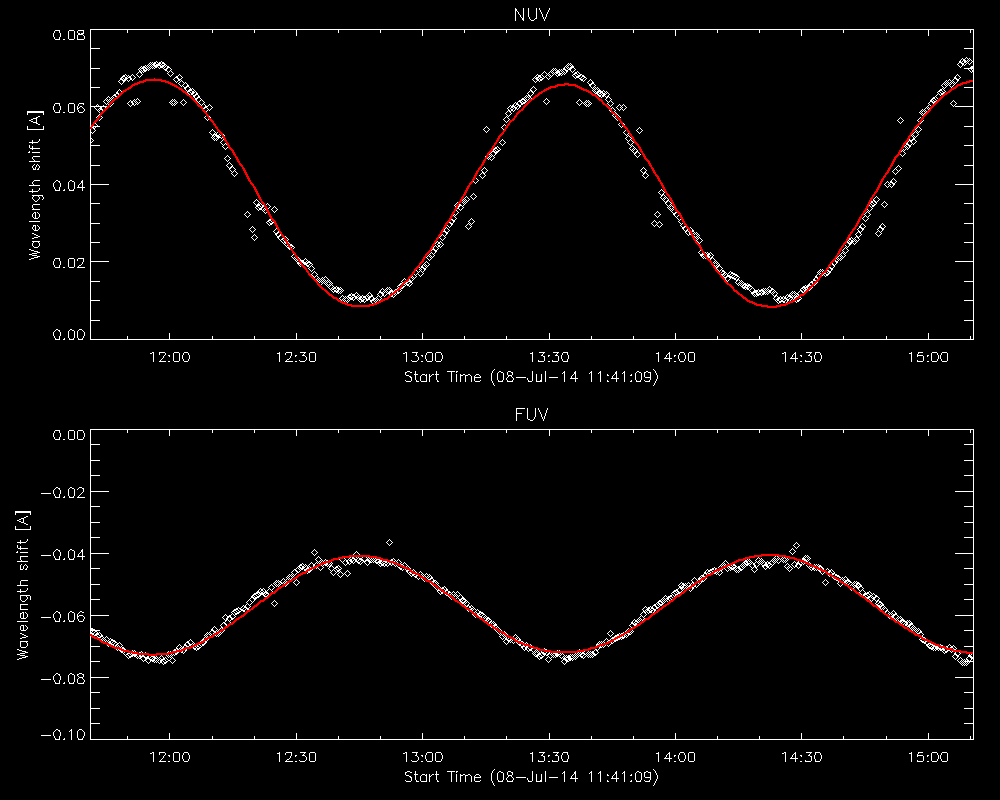
Fit to the orbital velocity/thermal shifts from iris_prep_wavecorr_l2.
Note
The smoothing of the wavelength variation assumes the IRIS orbital period. Shorter-timescale variations are sometimes evident; you can apply the shift of the individual measurements, or apply your own smoothing to the per-image measurements rather than using the smoothed corr_nuv and corr_fuv arrays if necessary.
To look at intensities at any given scan we only need to subtract this shift from the wavelength scale, but to look at the whole image at a given wavelength we must interpolate the original data to take this shift into account. Here is a way to do it (note that array dimensions apply to this specific set only!):
IDL> new_data = fltarr(536, 1092, 400, /n)
IDL> .r
for i=0, 399 do begin
   for j=0, 1091 do begin
       new_data[*, j, i] = interpol(data[*, j, i], wave + wavecorr.corr_nuv[i], wave)
   endfor
endfor
end
(This double loop may take a while to complete.)
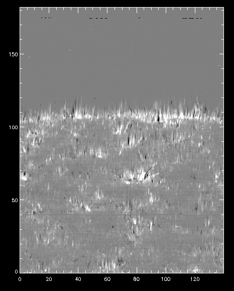
Once you have the calibrated data, we can compare again how it looks at the Mn I line wavelength:
IDL> pih, transpose(reform(new_data[350,*,*])), min=0, max=200, scale=[0.35,0.1667]
And now we can see that the intensity map is uniform along the solar disk:
Intensity at Mn I 280.2 nm line when orbital velocity and thermal drifts are accounted for.
We can use this calibrated data for example to calculate dopplergrams. A dopplergram is the difference between the intensities at two wavelength positions at the same (and opposite) distance from the line core. For example, at +/- 50 km/s from the Mg II k3 core. To do this, let us first calculate a velocity scale for the h line and find the indices of the -50 and +50 km/s velocity positions (here using the convention of negative velocities for up flows):
IDL> k_centre = 2796.32   ; mean position of k3
IDL> vel = (wave - k_centre) * 3e5 / k_centre
IDL> tmp = min(abs(vel - 50), i50p)  ; find index of -50 and 50 km/s
IDL> tmp = min(abs(vel + 50), i50m)
Now get the Dopplergram and plot it:
IDL> doppgr = transpose(reform(new_data[i50m, *, *] - new_data[i50p, *, *]))
IDL> pih, doppgr, min=-200, max=200, scale=[0.35, 0.1667]
Dopplergram for Mg II k at +/- 50 km/s.
7.3. Mg II spectral feature identification
In this tutorial we will measure the intensities and velocity shifts of the Mg II k3 and k2 features. We will make use of the iris_get_mg_features_lev2 procedure, which is included in the IRIS SSW package.
Here we will use the same dataset as for the tutorial IRIS xfiles and CRISPEX above. If you haven’t done so, start by downloading an IRIS dataset from 2013 December 26: follow this link and download the raster file (491 Mb). Download it to a directory of your choice. Unzip it, e.g. on a UNIX system:
% tar zxvf iris_l2_20131226_171752_3840007146_raster.tar.gz
We can calculate the properties of the Mg II k line in the following manner:
IDL> filename = 'iris_l2_20131226_171752_3840007146_raster_t000_r00000.fits'
IDL> iris_get_mg_features_lev2, filename, 3, [-40, 40], lc, rp, bp, /onlyk
(This will take a while.)
The output is saved in the arrays lc (line centre), rp (red peak), and bp (blue peak). To save time, we calculated only for the k line. We can then visualise both the derived velocities and intensities. For the intensities:
IDL> pih, transpose(reform(lc[0,1,*,*])), min=0, max=500, scale=[0.35,0.1667]
IDL> pih, transpose(reform(bp[0,1,*,*])), min=0, max=750, scale=[0.35,0.1667]
IDL> pih, transpose(reform(rp[0,1,*,*])), min=0, max=750, scale=[0.35,0.1667]
Intensity for the k3 peak from iris_get_mg_features.
and for the velocities:
IDL> pih, transpose(reform(lc[0,0,*,*])), min=-15, max=15, scale=[0.35,0.1667]
IDL> pih, transpose(reform(rp[0,0,*,*])), min=0, max=30, scale=[0.35,0.1667]
IDL> pih, transpose(reform(bp[0,0,*,*])), min=-30, max=0, scale=[0.35,0.1667]
Velocity shifts for the k3 peak from iris_get_mg_features.
As you can see, the code is not perfect at finding the positions of the spectral features in all pixels (see obvious black and white isolated pixels). Instead, it provides a reasonable estimate when the line profiles are well behaved, and a starting point to further analysis.
7.4. Time series analysis
In this tutorial we are going to work with spectra and slit-jaw images to study dynamical phenomena. The subject of this example is umbral flashes.
Start by downloading this IRIS dataset from 2013 September 2. Download the three slit-jaw files and the raster file (about 1 Gb in total) to a directory of your choice. Unzip all the files, e.g. on a UNIX system:
% gunzip *fits.gz
% tar zxvf *.tar.gz
Start sswidl and use the iris_files function to get a list of all the IRIS FITS files:
IDL> f = iris_files('./*')
   0  iris_l2_20130902_163935_4000255147_SJI_1330_t000.fits     123 MB
   1  iris_l2_20130902_163935_4000255147_SJI_1400_t000.fits     123 MB
   2  iris_l2_20130902_163935_4000255147_SJI_2796_t000.fits     123 MB
   3  iris_l2_20130902_163935_4000255147_raster_t000_r00000.fits  1 GB
You can now start an iris_obj with this list of files, but it must be reversed because iris_obj expects the spectral raster first:
IDL> d = iris_obj(reverse(f))
IDL> d->show_lines
Spectral regions(windows)
 0   1335.71   C II 1336
 1   1349.43   Fe XII 1349
 2   1351.66   Cl I 1352
 3   1355.60   O I 1356
 4   1393.78   Si IV 1394
 5   1402.77   Si IV 1403
 6   2786.14   2786
 7   2796.20   Mg II k 2796
 8   2830.93   2830
Loaded Slit Jaw images
 0   SJI_1330
 1   SJI_1400
 2   SJI_2796
We can now get the data and wavelength for the Mg II and C II windows, and the array of times (since the start of the observations):
IDL> data_c = d->getvar(0, /load)
IDL> wave_c = d->getlam(0)
IDL> data_mg = d->getvar(7, /load)
IDL> wave_mg = d->getlam(7)
IDL> times = d->gettime()
For this dataset the spectral cadence is about 3 seconds. The Mg II k3 core is located around wavelength pixel 103. We can use this information to make a space-time image of the Mg II k3 wavelength:
IDL> pih, transpose(reform(data[103,*,*])), min=0, max=200, scale=[3./60.,0.1667]
The result can be seen below, with the x axis in minutes and the y axis in arcsec.
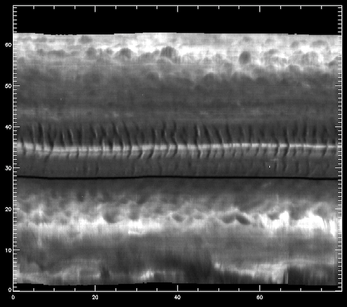
Space-time diagram of the intensity at around the Mg II k3 core.
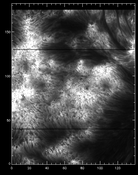
The middle section between 30”-40” is on the umbra of a sunspot, even though it is not obvious from this image. One can see very clearly the umbral oscillations, with a clear regular pattern of dark/bright streaks. Let us now load the 1400 slit-jaw and plot it for context:
IDL> sji = d->getsji(1)
IDL> pih, sji[*,*,0], min=0, max=200, scale=[0.1667,0.1667]
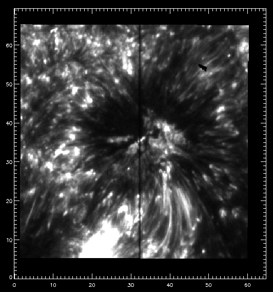
First SJI 1400 image of the observing sequence.
The slit pixel 220 is a location on the sunspot’s umbra. We will use it to get some plots. For example, let’s plot the k3 intensity (spectral pixel 103 of data_mg) and the core of the brightest C II line (spectral pixel 90 of data_c) vs. time in minutes (showing first 10 minutes only):
IDL> plot, times/60., data_mg[103, 220, *], xrange=[0, 10], yrange=[0, 80], $
       /xst, /yst
IDL> oplot, times/60., data_c[90, 220, *] * 2, linestyle=1
In the above we are multiplying the C II data by two to get the two lines closer. Image now you wanted to compare these oscillations with the intensity on the slit-jaw. How to do it? The slit-jaws are tipically taken at a different cadence, so you will need to load the corresponding time array for the 1400 slit-jaw:
IDL> times_sji = d->gettime_sji(1)
IDL> help, times_sji
TIMES_SJI      DOUBLE    = Array[400]
This is the time in seconds since the start of the observations, so comparable to the array times, which holds the same quantity for the spectra. Armed with this, we can now plot the SJI intensity for a pixel close to the slit at the same y position (index 220):
IDL> oplot, times_sji/60., sji[220, 190, *], linestyle=2
The resulting plot can be found below. You are now ready to explore all the correlations, anti-correlations, and phase differences.
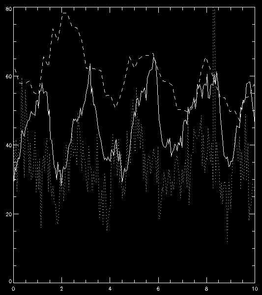
Intensity vs. time in minutes for an umbral flash oscilation, for Mg II k3 (solid), C II 1335 core (dotted) and 1400 slit-jaw (dashed).
7.5. Other tutorials
Notes and videos are also available from tutorials held at IRIS workshops. Some of these are based on the above tutorials and focused on IRIS data, while others cover related topics such as radiative transfer and analysing output from Bifrost simulations:
7.5.1. Tutorials from IRIS-4 workshop
7.5.2. Tutorials from IRIS-7 workshop
- Introduction to IRIS data analysis: materials
- Bifrost simulations: materials 1 and materials 2
- Operation of IRIS: materials
- Flare simulations: materials
- UV Spectroscopy: materials