3. Reading and browsing IRIS-SDO-Hinode co-aligned data cubes
3.1. Reading level 2 co-aligned SDO and Hinode datasets
One of the main advantages of the newly created data cubes is their structure, which is the same as IRIS level 2 SJI FITS files. This common structure means that all data can be examined using the IRIS SolarSoft package. Therefore, to read SDO and Hinode data cubes into memory, one can follow the same instructions as in the case of IRIS SJI data cubes. For example, we can easily visualize SDO and Hinode datasets using iris_xfiles and iris_ximovie, since they are recognized by IRIS software as slit-jaw files. The figure below shows iris_ximovie widgets displaying the Hinode/SOT (a), IRIS (b) and SDO/AIA (c) data cubes from the previous chapter as slit jaw sequences.
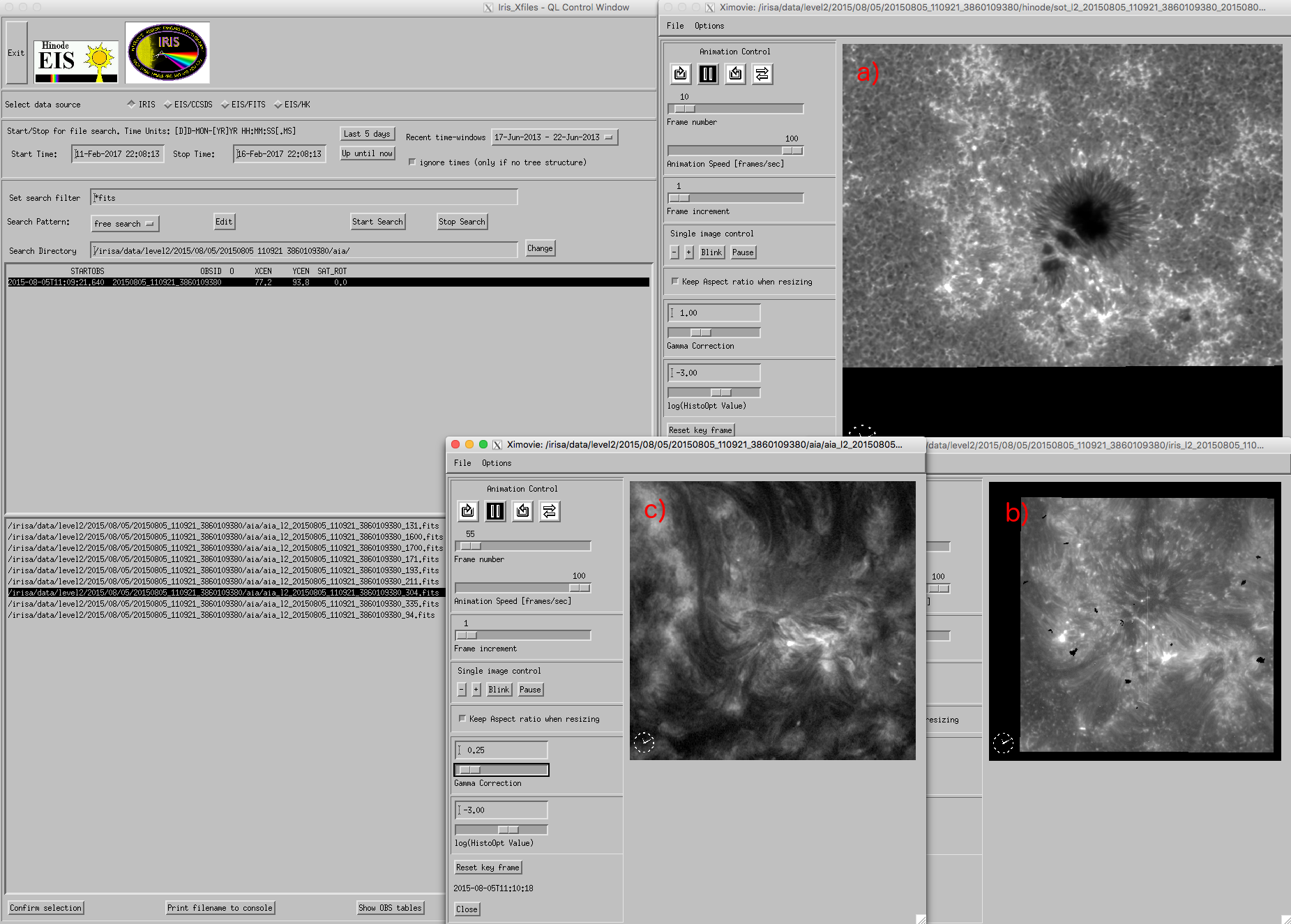
``iris_ximovie`` showing selected Hinode (a), IRIS (b) and AIA (c) data sequences. ``iris_ximovie`` windows has been resized for a better arrangement of the panels.
To read the data we can use read_iris_l2 routine. We will continue with the same IRIS observational sequence we used until now and load into memory the associated co-aligned Hinode Ca II H filtergrams:
IDL> dir_sot='/irisa/data/level2/2015/08/05/20150805_110921_3860109380/hinode/'
;find Hinode/SOT files
IDL> f_sot=iris_files(path=dir_sot) ;find Hinode/SOT files
0  (...)sot_l2_20150805_(...)_CaIIHline_FG.fits     292 MB
1  (...)sot_l2_20150805_(...)_Gband4305_FG.fits      28 MB
;read Ca II H data into memory and retain NULL images
IDL> read_iris_l2, f_sot[0], index, data, /silent, /keep_null
IDL> help, data
DATA FLOAT = Array[631, 601, 202]
In the same way we can read AIA data cubes:
IDL> dir_aia='/irisa/data/level2/2015/08/05/20150805_110921_3860109380/aia/'
;find all AIA level 2 FITS files
IDL> f_aia=iris_files(path=dir_aia)
0  (...)aia_l2_20150805_110921_3860109380_131.fits     453 MB
1  (...)aia_l2_20150805_110921_3860109380_1600.fits     226 MB
2  (...)aia_l2_20150805_110921_3860109380_1700.fits     224 MB
3  (...)aia_l2_20150805_110921_3860109380_171.fits     453 MB
4  (...)aia_l2_20150805_110921_3860109380_193.fits     453 MB
5  (...)aia_l2_20150805_110921_3860109380_211.fits     453 MB
6  (...)aia_l2_20150805_110921_3860109380_304.fits     453 MB
7  (...)aia_l2_20150805_110921_3860109380_335.fits     453 MB
8  (...)aia_l2_20150805_110921_3860109380_94.fits     453 MB
;read AIA 1700 observations
IDL> read_iris_l2,f_aia[2], index, data, /keep_null
IDL> help, data
DATA FLOAT = Array[392, 382, 786]
In both examples, IDL variable data contains the corresponding images, while the index variable stores the associated headers as an IDL structure. The index variable contains standard FITS header keywords for Hinode and SDO/AIA observations, respectively. In addition, the new co-aligned data cubes headers have additional keywords. Their purpose is to provide specific information related to data reduction process, quality keywords, associated web pages, etc. For example the co-aligned Hinode data cubes have among others, two new keywords that together form the link to the corresponding HCR page:
IDL> print, strjoin([index[0].sotlink1, index[0].sotlink2])
http://www.lmsal.com/hek/hcr?cmd=view-event&event-id=ivo%3A%2F%2Fsot.lmsal.com%2FVOEvent%23VOEvent_ObsS2015-08-04T21%3A04%3A00.000.xml
It is important to note that both Hinode and AIA headers have four keywords defining the time range when the observations were recorded:
DATE_OBS- the time of the first available exposure in the respective Hinode or SDO level 2 file;DATE_END- the time of the last exposure;STARTOBS- gives the time when the coordinated IRIS OBS started;ENDOBS- the time when the coordinated IRIS OBS ended.
3.2. Browsing co-aligned SDO and Hinode data cubes with CRISPEX
Co-aligned SDO/AIA and Hinode/SOT datasets cannot be converted into level 3 data since they do not include spectroscopic data, but it is possible to use them in CRISPEX along with level 3 IRIS image and spectral cubes. Level 3 IRIS data can be generated either via iris_xfiles or iris_make_fits_level3 routine. Here we will demonstrate it using the latter option. First we select IRIS raster files and check the spectral windows indices:
IDL> dir='/irisa/data/level2/2015/08/05/20150805_110921_3860109380/'
;select IRIS raster files
IDL> f = iris_files('/*raster*.fits', path=dir)
;extract the spectral windows and print them
IDL> wi=iris_obj(f[0])
IDL> wi->show_lines
Spectral regions(windows)
0   1335.71   C II 1336
1   1343.26   1343
2   1349.43   Fe XII 1349
3   1355.60   O I 1356
4   1402.77   Si IV 1403
5   2832.79   2832
6   2826.73   2826
7   2814.51   2814
8   2796.20   Mg II k 2796
In this example, we will proceed with C II, Si IV 1403, and Mg II k spectral windows. Now we select IRIS SJI fits files and then call iris_make_fits_level3 procedure to generate level 3 data that will be saved to the '~/Desktop/' folder:
;select IRIS SJI files
IDL> s = iris_files('*SJI*.fits', path=dir)
;create IRIS level 3 data
IDL> iris_make_fits_level3, f, [0, 4, 8], /sp, sjifile=s[0], wdir='~/Desktop/'
After selecting the newly generated level 3 data cubes, we can use CRISPEX to visualize the data:
;select IRIS level 3 data
IDL> cd, '~/Desktop/'
IDL> f = iris_files('/*l3*.fits')
;call crispex
IDL> crispex, f[0], f[1], sjicube=s[0]
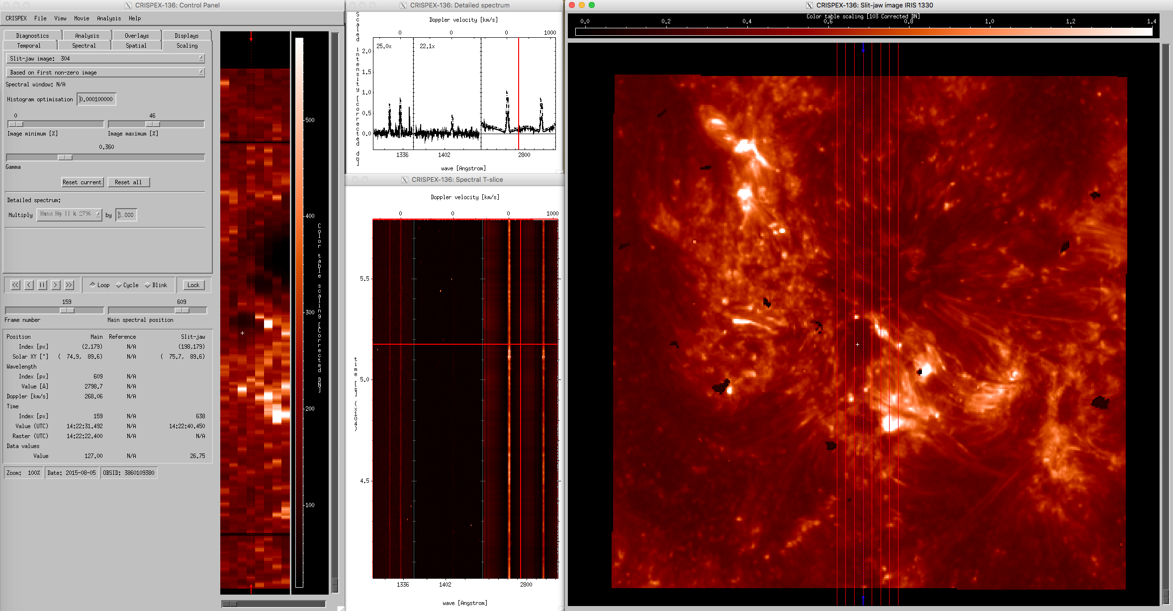
``CRISPEX`` windows for IRIS OBSID 20150805_110921_3860109380 with large coarse 8-step raster. The middle column shows spectral windows (upper panel) and λ-t diagrams (bottom panel). IRIS SJI 1330 Å are used as reference images (right panel).
Since co-aligned SDO and Hinode datasets have the same structure as IRIS SJI level 2 data, they can be used as an argument in CRISPEX. For example, if we want to examine simultaneously IRIS raster files and SDO/AIA 304 Å observations, then we can use the following command:
crispex, f[0], f[1], sjicube=f_aia[6]
The resulting CRISPEX widget is shown in the figure below (left panel). If we want to explore IRIS rasters and Hinode Ca II H observations (right panel), then we can call:
IDL> crispex, f[0], f[1], sjicube=f_sot[1]

``CRISPEX`` windows for IRIS OBSID 20150805_110921_3860109380. The left panel shows AIA and the right panel SOT data as reference images.
It is possible to simultaneously use up to six data cubes as reference cubes when sjicube keyword is fed by a vector of indices, for example:
IDL> crispex, f[0], f[1], sjicube=[s[0], s[1],...]