3. Diagnostics based on the Mg II h&k lines
3.1. Introduction
The spectral lines Mg II h&k are considered as some of the best lines to recover information from the chromosphere. These lines, among many others, are located and observed by IRIS in the near Ultraviolet (NUV) spectral range. Table 3.1 shows the main specifications of IRIS spectrograph (SG) in the NUV, and at what temperature range these IRIS observations are sensitive.
| Band | Wavelength (Å) | Dispersion (mÅ/pix) | Effective area (cm2) | Temperature (log T) |
|---|---|---|---|---|
| NUV | 2782.7–2851.1 | 25.46 | 0.2 | 3.7–4.2 |
Other interesting lines are in the IRIS NUV SG spectral range. Some of them may be used as diagnostics in the photosphere as it is explained in Section 1.
In this tutorial, we first explain how the Mg II h&k lines are formed, where they are sensitive in the solar atmosphere, and their profile features. Then, we explain how we can find these profiles features and the limitations of that search. Finally, we show how to obtain physical information from the profile features.
3.2. The Mg II h&k lines
We focus our attention in the Mg II h & k lines. These lines are the more prominent lines in the IRIS NUV spectral range.
3.2.1. Formation of the Mg II h&k lines
Table 3.2 shows several physical values related with the formation of these lines. A graphical representation (Grotrian diagram) of these transitions are given in Fig. 3.1.
Solar Jargon
|
Wavelength
(Å)
|
\(E_{lower} - E_{upper}\)
(eV)
|
Lower Level
Config., Term, J
|
Upper Level
Config., Term, J
|
Solar Jargon
|
|---|---|---|---|---|---|
| Mg II UV Triplet 1 | 2790.776 | 4.422431 - 8.863762 | \(2p^{6}3p\ \ ^{2}P^{o}\ \ 1/2\) | \(2p^{6}3d\ \ ^{2}D\ \ 3/2\) | Mg II UV Triplet 1 |
| Mg II k | 2795.528 | 0.000000 - 4.433784 | \(2p^{6}3s\ \ ^{2}S\ \ 1/2\) | \(2p^{6}3p\ \ ^{2}P^{o}\ \ 3/2\) | Mg II k |
| Mg II UV Triplet 2 | 2797.930 | 4.433784 - 8.863762 | \(2p^{6}3p\ \ ^{2}P^{o}\ \ 3/2\) | \(2p^{6}3d\ \ ^{2}D\ \ 3/2\) | Mg II UV Triplet 2 |
| Mg II UV Triplet 3 | 2797.998 | 4.433784 - 8.863654 | \(2p^{6}3p\ \ ^{2}P^{o}\ \ 3/2\) | \(2p^{6}3d\ \ ^{2}D\ \ 5/2\) | Mg II UV Triplet 3 |
| Mg II h | 2802.704 | 0.000000 - 4.422431 | \(2p^{6}3s\ \ ^{2}S\ \ 1/2\) | \(2p^{6}3p\ \ ^{2}P^{o}\ \ 1/2\) | Mg II h |
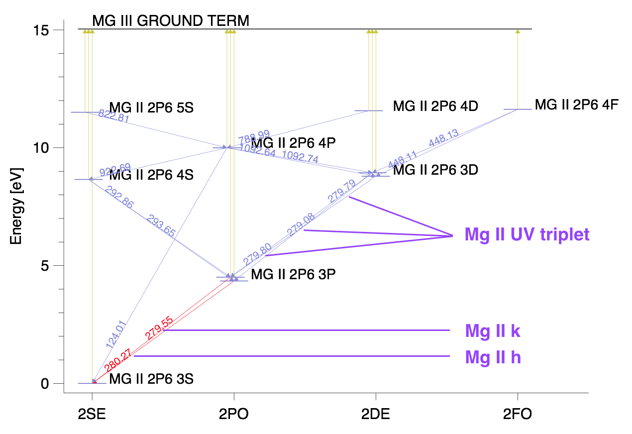
Fig. 3.1 Partial Grotrian diagram showing 10-level plus continuum Mg II atomic model and some of the transitions between these levels and the levels and the continuum. Mg II h&k lines and Mg II UV triplet are specifically indicated. Source Leenaarts et al. 2013.
3.2.2. Profile features of the Mg h&k lines
We are going to use the spectral features in the Mg II h&k lines to derive some physical proxies from the chromosphere. First, we have to get familiarized with these features and their nomenclature. Fig. 3.2 shows a spatially averaged profile in the quiet sun observed by IRIS NUV SG (left panel), and the zoomed-in Mg II h&k lines (right panel). Around the core or central depression of the Mg II h&k lines (marked with thick-dashed lines in the left panel), we can distinguish 2 peaks. The values at these three locations (the peaks and the core) and two other ones located in the wings of the lines are the tools we will use to infer some physical proxies.
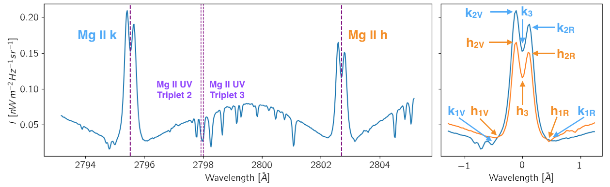
Fig. 3.2 Spatially-averaged Mg II h&k profiles in the quiet sun (top), plage (center), and X-flare ribbon (bottom). Vertical lines mark the center of the Mg II h&k lines and two of the Mg II UV triplet (see Table 3.2).
For the Mg II k line, starting counting from the wavelengths in the violet (left) side of the line , we found: the minimum of the wing, what we denote by \(k_{1V}\); the first peak, \(k_{2V}\); the core of the line \(k_{3}\); the second peak, what is located in the red (right) side with respect to the core (or central depression) of the line, \(k_{2R}\); and finally , the minimum of the wing located in the red side with respect to the core, \(k_{1R}\). Similar notation is used for Mg II h line (see left panel in Fig. 3.2, orange). We notice that these locations are profile features and they are not defined for a particular or ad-hoc defined wavelength but for the shape of these lines. Therefore, we should distinguish between the intensity and the wavelength position of these profile features.
We use the intensity of these profile features to diagnose temperatures.
We use the wavelength of these profile features (or separation between them) to diagnose velocities or velocity gradients.
We use the ratio between the difference of peak intensities and sum of peak intensities to determine downflows or upflows.
3.2.2.1. Basic analysis of the profile features
At a glance, we may distinguish two basic signatures in many Mg II h&k lines.
Higher mountains and higher valley
As we can see in the top panel, the intensity in the peaks and the cores of the Mg II k line is higher than for the peaks and the core in the Mg II h line. This is because the \(k\) line has an oscillator strength twice larger than the \(h\) line , and optical depth \(\tau = 1\) in the peaks of the \(k\) line is located at larger heights, where the source function is larger, than for the \(h\) line. As a consequence, the emission in the \(k\) peaks is (usually) larger than in the \(h\) peaks.
Downflows or upflows?
Another feature we can distinguish in both profiles in the top panel of Fig. 3.5 is the difference in intensity between \(k_{2V}\) and \(k_{2R}\) (similarly for the \(h\) line). In the middle panel, the intensity of \(k_{2V}\) is lower than the intensity of \(k_{2R}\) (similarly for the \(h\) line). The difference between the peaks of the same line may be explained by a downflow (called as inflow in the left pane in Fig. 3.3) or an upflow (called as outflow in the right panel).
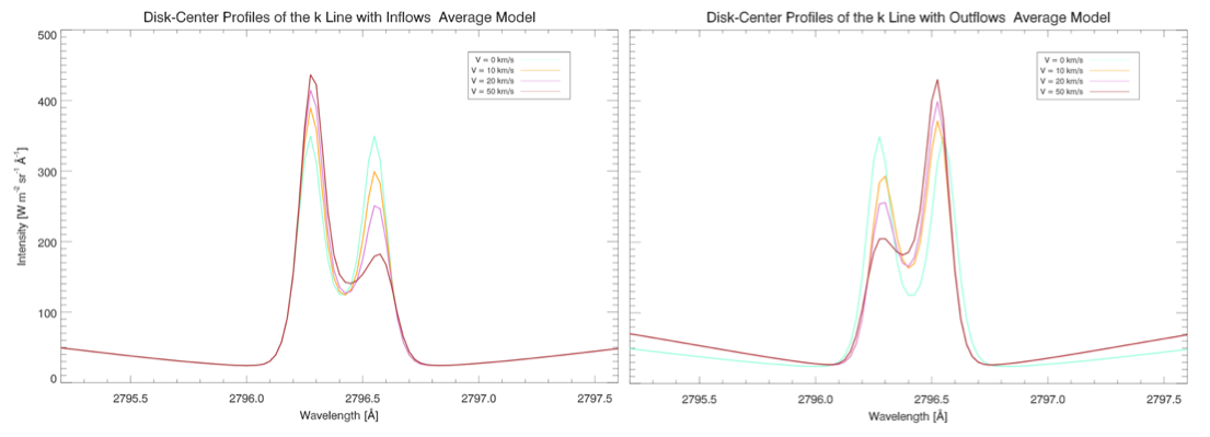
Fig. 3.3 Synthetic Mg II k profile at disk-center considering inflows (left) or outflows (right). See Source E. Avrett.
3.2.3. Where the Mg II h&k lines are sensitive?
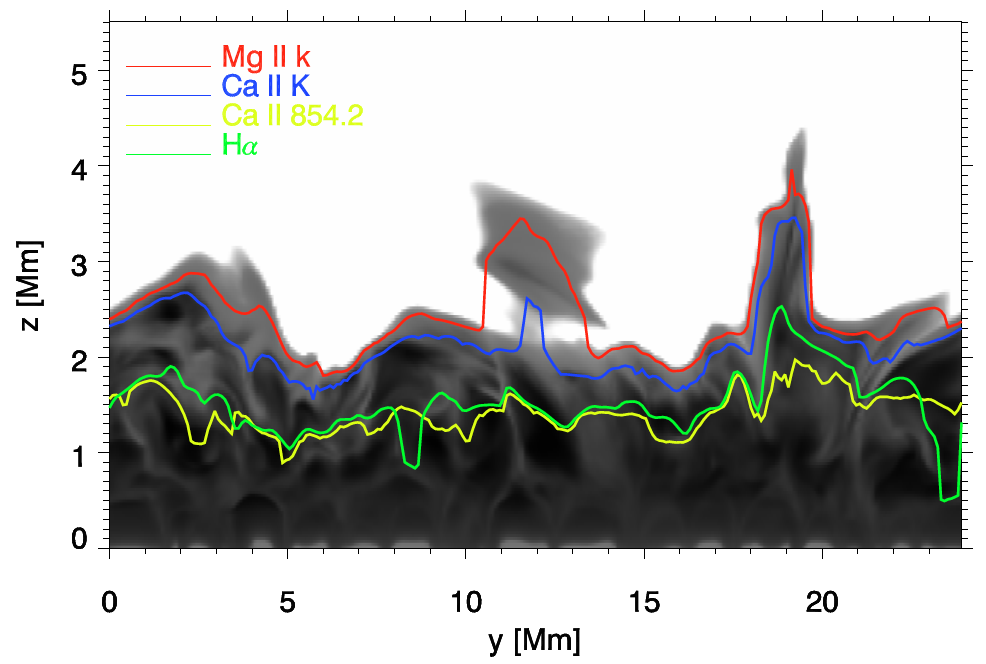
The Mg II h&k lines are formed in the chromosphere. This sentence is as true as imprecise. We prefer to say a line is sensitive to a value of the magnetic field and the hydrodynamics conditions, or in a fewer words, to some atmosphere conditions at a certain region or optical depth.
That being said, it has shown that the Mg II h&k lines are formed in a corrugated region with optical depth equals to 1 located in the upper chromosphere (see left panel in Table 3.3). More precisely, the profile features \(k_3\) and \(h_3\) are formed in the upper chromosphere, about 200 km below the transition region (TR). The difference between the \(k_3\) and \(h_3\ \tau=1\) height is about 50 km (Pereira et al. (2013)), while the peaks (\(k_{2V/R}\) and \(h_{2V/R}\)) are formed in the middle chromosphere, being the difference between \(k_{2V}\) and \(k_{2R}\) about 350 km. Finally, the average \(\tau =1\) height for \(k_{1V}\) is located in the photosphere. Table 3.3 summarizes these values for the \(k\) line.
 |
Profile Feature | Average \(\tau=1\) height [km] |
| \(k_{3}\) | 2200 (upper chromosphere). 200 below TR | |
| \(k_{2V}\) | 1550 (mid chromosphere) | |
| \(k_{2R}\) | 1200 (mid chromosphere) | |
| \(k_{1V}\) | 600 (mid photosphere) |
3.2.4. Radiation field, thermodynamics, and geometry: 1D or 3D? CRD or PRD?
Our knowledge about the Mg II h&k lines has grown since the IRIS project was accepted to be launched. A tremendous effort has been done by the solar community (specially at LMSAL, University of Oslo, and Institute for Solar Physics at Stockholm University) to understand the behavior of these lines. Our current knowledge comes mainly from the analysis of synthetic profiles obtained from state-of-the-art 3D numerical simulations and the recent IRIS observations. Another important constrain to reproduce the observed profiles is to consider the conditions of the interaction between the radiation field and the matter in the chromosphere.
For the Mg II h&k lines we have to consider this interaction in non-local thermodynamic equilibrium (non-LTE) with partial redistribution (PRD, see Milkey & Mihalas 1974). Until very recently, we were not able to simulate simultaneously all the conditions needed to successfully reproduce the Mg II h&k lines: 3D MHD non-LTE + PRD. Sukhorukov & Leenaarts (2017) synthesized Mg II h&k lines using different codes (RH and Multi3D) and complete redistribution (CRD) or PRD. Their main conclusions are:
- 1D PRD approximations reproduce the wavelength positions of all the profile features correctly. That means, the wavelength positions corresponding to \(k_{1V/R}, k_{2V/R}, k_{3}\) and similarly for the h line.
- 1D PRD can be used to compute the intensity in the inner wings, (\(k_{1V/R}\) and \(h_{1V/R}\)), specially \(k_{1R}\) and \(h_{1R}\).
- The emission peaks (\(k_{2V/R}\) and \(h_{2V/R}\)) are affected by both 3D and PRD effects. Therefore, both effects have to be considered simultaneously to properly reproduce these profiles features.
- The intensity at the core of the lines \(k_{3}\) and \(h_{3}\) can be accurately calculated using 3D+PRD at the center of the solar disk, but not towards the limb.
- Accurate quantitative modeling from the whole line profile and its center-to-limb variation requires 3D+PRD.
Some of these ideas are shown in Fig. 3.4.
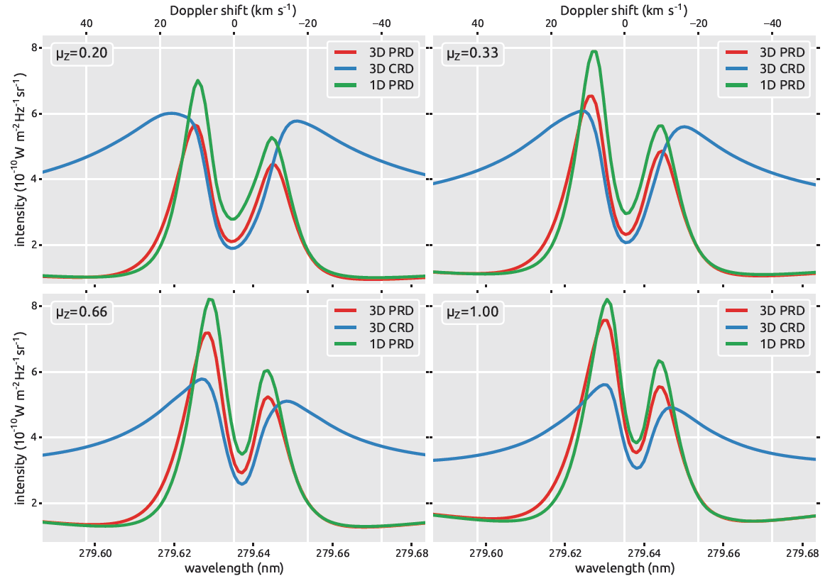
Fig. 3.4 Mg II k line profiles for spatially averaged intensity in 3D PRD (red), 3D CRD (blue), and 1D PRD (green) computed at different Z angles in the 3D Bifrost model atmosphere. Source Sukhorukov and Leenaarts (2017)
3.2.5. Using the profile features of the Mg II h&k lines to diagnose the chromosphere
Now that we have a better understanding about how the Mg II h&k lines are formed, where they are sensitive, and their profile features, we can use this knowledge to infer physical parameters of the region(s) where these lines are observed.
3.2.6. Automatic identification of the profiles features of Mg II h&k profiles observed by IRIS
The Mg II h&k profile showed in Fig. 3.2 is a spatially-averaged profile in the quiet sun. The profile features in that profile are easy to identify, and, therefore, the diagnosis based on these features will work correctly. However, other Mg II h&k profiles may barely show the profile features or even do not show them at all, making their identification a challenging task either for the human eye or an identification code. Fig. 3.5 shows the same profile that Fig. 3.2, i.e. spatially averaged profile in the QS (top), and two spatially-averaged Mg II h&k lines profiles in the outer (middle panel) and the top (bottom panel) of a ribbon X-class flare. As we can see, in these two last profiles some the profile features are hard to distinguish or even not present at all, as it happens with the top of the ribbon flare, where only the \(k_{3}\) profile feature can be identified. Fig. 3.5 shows an attempt to fit these profiles as the sum (orange) of 7 Gaussian profiles (color-dotted lines). Although the fit is quite good in the three cases, to find the locations of the profile features from the Gaussian profiles may be a relatively easy task (e.g. QS and outer of the flare ribbon), or a hard task (e.g. top of the flare ribbon profile).
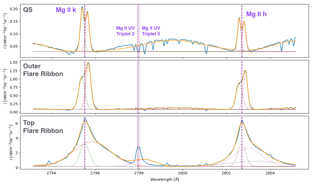
Fig. 3.5 In blue, spatially-averaged Mg II h&k profiles observed in the quiet sun (top), in the outer (middle), and the top (bottom) of a ribbon X-class flare. In orange, the fit of these profiles using 7 Gaussian profiles: 2 for the further wings in the left and the right of the \(k\) and \(h\) line respectively; 2 for the \(k\) line; 1 for the bump between the \(k\) and \(h\) line; an other 2 Gaussian profiles for the \(h\) line.
A method to find the profiles features of Mg II h&k profiles observed by IRIS has been developed by Dr. T. M. D. Pereira. This method and other available diagnostic tools are available in the SolarSoftware package. A detailed guide about how to analyze the IRIS data may be found at the ITN26. In Section 8.3 of ITN26 it is very well explained how to obtain the location of the profiles features, their intensity, and the Doppler velocities associated to their locations (or their differences). We address to the interested reader to follow the steps described there to compute these values and quantities. In this tutorial, we explain the justification of the methods used to diagnose the physical parameters from the profile features.
3.3. Calculating velocities
As we have already mentioned, we use the position of the profile features to determine velocities, more precisely the vertical component of the velocity (\(v_{z}\)), the gradient of \(v_{z}\), or the average vertical velocity. These magnitudes are referred to the profile feature(s) used to calculate it, e.g. \(\Delta v_{k_2}\). Therefore, that velocity may be considered as a proxy in the region where that profile feature is formed.
3.3.1. Using \(k_{3}\) and \(h_{3}\)
Fig. 3.6 shows (linear) correlation between the Doppler shift of the \(k_{3}\) and \(h_{3}\) and the vertical component of the velocity at their respective \(\tau = 1\) height. Being Doppler shift of the \(k_{3}\)
\(\Delta v_{k_3} = \frac{\lambda_{k_3} - \lambda_{k_{0}}}{\lambda_{k_0}} c\)
with \(c\) the speed of light, and \(\lambda_{k_0}\) the rest-frame line-center wavelength (see Table 3.2).
Therefore, knowing the spectral shift of the these profile features respect to their rest position will give us a rather accurate value of \(v_{z}\) in the upper chormosphere, i.e. where these profiles feature are formed (see Table 3.3).
All in all, we may say \(\Delta v_{k_3}\) is a very good proxy of \(v_{z}\) in the upper chromosphere, that is, at \(\tau_{k_{3}}=1\) height (see Table 3.3).
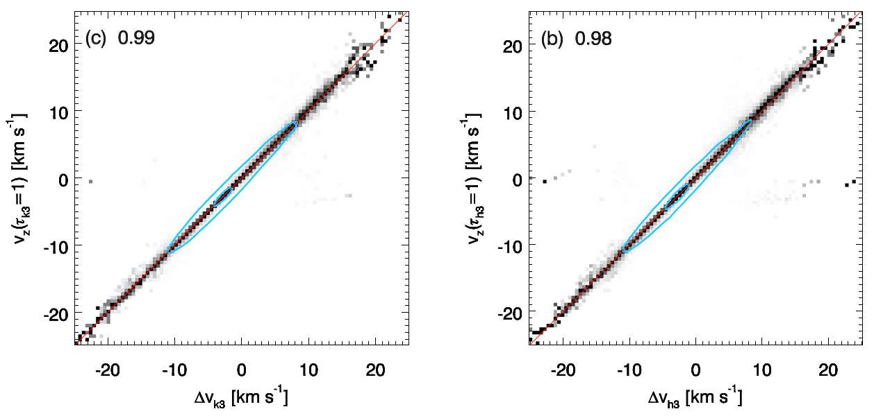
Fig. 3.6 Scaled joint probability density functions (JPDF) of the Doppler shift of \(k_{3}\) and \(h_{3}\) and the vertical component of the velocity at the region where \(\tau = 1\) for these lines. Source Leenaarts et al. (2013b).
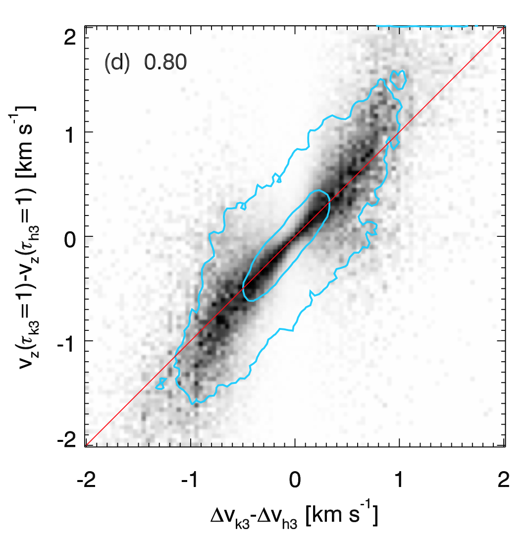
Fig. 3.7 Source Leenaarts et al. (2013b).
Fig. 3.7 shows the scaled JPDF of the difference between the Doppler shift of \(k_{3}\) and \(h_{3}\) and the difference between the vertical component of the velocity at the region where \(\tau = 1\) for these lines.
A gradient in the vertical component of the velocity, i.e. vertical acceleration, in the upper chromosphere may be calculated as the difference between the Doppler shift of \(k_{3}\) and \(h_{3}\) profile features. Leenaarts et al. (2013b) show that although the correlationship between \(\Delta v_{k_{3}} - \Delta v_{h_{3}}\) and \(v_{z}(\tau_{k_{3}} = 1) - v_{z}(\tau_{h_{3}} = 1)\) is not as good as in the relationship between \(\Delta v_{k_3}\) and \(v_{z}(\tau_{k_{3}} = 1)\) (r = 0.80, see Fig. 3.7), \(\Delta v_{k_{3}} - \Delta v_{h_{3}}\) is a valid proxy to determine the sign and magnitude of the velocity difference in the upper chromophere.
3.3.2. Using the peaks \(k_{2VR}\) and \(h_{2VR}\)
We are going to use three different observable quantities derived from the profile features:
- peak separation (between peaks at the same line), e.g. \(\Delta \lambda_{k} = (\lambda_{k_{2V}} - \lambda_{k_{2R}})\), or in velocity units \(\Delta v_{k_2} = \frac{\lambda_{k_{2V}} - \lambda_{k_{2R}}}{\lambda_{k_0}}c\)
- average Doppler shift, e.g. \(\Delta v_{k_{0}} = - \frac{1}{2} \frac{c}{\lambda_{k_{0}}}\big[(\lambda_{k_{2V}} - \lambda_{k_{0}})+(\lambda_{k_{2R}} - \lambda_{k_{0}})\big]\)
- intensity radio of the peaks, e.g. \(R_{k} = \frac{I_{k_{2V}} - I_{k_{2R}}}{{I_{k_{2V}} + I_{k_{2R}}}}\)
3.4. Calculating temperatures
At the height where \(\tau =1\) for \(k_3\) and \(h_{3}\) the source function is decoupled from the thermal local conditions (see lower-right panel in Fig. 7 in Leenaarts et al. (2013a)). Therefore, the intensity in those profile features are not valid to calculate temperature. However, at \(\tau =1\) height for the peak profile features there is some coupling between the source function and the thermal conditions (see lower-left panel in Fig. 7 in Leenaarts et al. (2013a)). We will use the intensity in these profile features to calculate the temperature in the mid chromospere. Thus, the intensity in the peaks, \(I_{k_{2}}\) and \(I_{h_{2}}\) can be converted to radiation (or brightness) temperature, \(T_{rad}\) or \(T_{brigh}\), which can be considered as a good proxy for \(T_gas (\tau_{k_2} = 1)\).
This proxy has been proven using numerical simulations by Leenaarts et al. (2013b) (see Fig. 3.8), and temperatures obtained by the inversion of the Mg II h&k lines using STiC (de la Cruz Rodríguez et al. (2016)) by Gošić et al. (2018) (see Fig. 3.9).
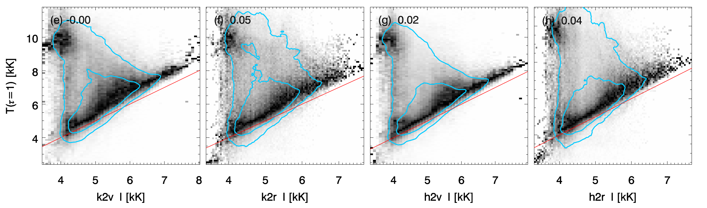
Fig. 3.8 Relationship between the intensity in the \(k_{2}\) and \(h_{2}\) and the temperature at the corresponding \(\tau =1\) height. Source Leenaarts et al. (2013a).
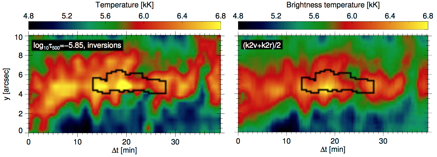
Fig. 3.9 Relationship between the average intensity in the \(k_{2}\) peak and the temperature at \(log \tau_{500} = -5.8\). Source Gošić et al. (2016).
3.5. Summary
The features in the profile of the Mg II h&k lines have revealed as very good tools to recover valuable information in the mid and upper chromosphere. Table in Table 3.4 summarizes the usage we may do with the observables calculated from these profile features.
Note
Despite careful calibrations and data processing, some of the calculations in this tutorial my be affected by minor problems in the final IRIS data product. Many of those problems are corrected in the recent mission-long data reprocessing completed in September 2017, while some of them still remain uncorrected. However, the majority of the problems, especially those ongoing ones, have negligible to minor impact on science data in general. A complete list of IRIS idiosyncrasies can be found in ITN 40 IRIS Data Idiosyncrasies
| Spectral Observable | Atmospheric Property |
|---|---|
| \(\Delta v_{k3}\) or \(\Delta v_{h3}\) | Upper chromospheric velocity |
| \(\Delta v_{k2}\) or \(\Delta v_{h2}\) | Mid chromospheric velocity |
| \(\Delta v_{k3} - \Delta v_{h3}\) | Upper chromospheric velocity gradient |
| \(k\) or \(h\) peak separation | Mid chromospheric velocity gradient |
| \(k_{2}\) or \(h_{2}\) peak intensity | Chromospheric temperature |
| \((I_{k2v}-I_{k2r})/(I_{k2v}+I_{k2r})\) | Sign of velocity above \(z(\tau=1)\) of \(k_{2}^{\text{a}}\) |
Note
The table above represents a simplified view and all correlations above have scatter. \(^{\text{a}}\) Likewise for the \(h_{2}\) peaks.