2. Formation of optically thin lines
This section aims to provide a basic overview of the atomic processes which give rise to the UV optically-thin line spectra observed by IRIS and some of the tools to derive important atomic physics parameters for the IRIS lines. For a more complete review on solar UV spectroscopy, the reader is referred to e.g. the book by Phillips et al. 2009 or the recent review by Del Zanna & Mason 2018, LRSP, 15, 5.
The intensity of an emission line strongly depends on:
- the number of emitting ions in the z-th ionization state of the element: \(X^\textrm{+z}\)
- the fraction of the ions \(X^\textrm{+z}\) which are in an energy level j giving rise to a particular spectral line: \(X^\textrm{+z}_\textrm{j}\)
For each ion in the solar plasma, there is a continuous interplay between the processes that change its ionization state (ionization/recombination, see Sect.2.1) and processes that populate/depopulate its excited levels (excitation/de-excitation, see Sect.2.2). In the low density plasma in the upper solar atmosphere, the timescales for ionization and recombination are usually much longer than those for excitation and de-excitation, so that the two sets of processes can often be de-coupled (e.g. Mariska 1992, Del Zanna & Mason 2018, LRSP, 15, 5). The intensity of an optically-thin line is proportional to the product of the contribution function, which contains the information on the relevant atomic processes, and the emission measure, which is determined by the physical conditions of the local plasma (see Sect.2.3). The freely available CHIANTI atomic database (Dere et al. 1997, A&AS, 125, 149, Del Zanna et al. 2015, A&A, 582, 56, see also the CHIANTI user guide ) provides a comprehensive set of atomic data covering the UV and X-ray wavelength ranges along with IDL routines to calculate the emission of optically thin, collisionally-dominated plasma for equilibrium conditions. A Phython version of CHIANTI is also available here.
It should be noted that the atomic processes are often evaluated assuming that the emitting plasma is in equilibrium conditions. However, during transient heating phenomena or in inhomogeneous plasma conditions, this assumption might not be longer valid. The most important non-equilibrium conditions which can be found in the solar atmosphere (i.e. non-equilibrium ionization and non-thermal equilibrium) will be briefly discussed in Sect. 2.4.
2.1. Excitation and de-excitation of atomic levels
In the upper solar atmosphere, the most important contributors to the level excitation are collisions between ions and free electrons (e.g. Phillips et al. 2009). By colliding with an electron, an ion can be excited from a lower energy state i to a higher one j:
Other processes, such as proton-ion collisions and photo-excitation, can also contribute to change the ion energy state but are usually less important (however, see e.g. Seaton 1964, MNRAS, 127, 191, Doschek 1971, ApJ, 170, 573).
Spontaneous radiative decay and collisional de-excitations are the main de-excitation mechanisms:
where \(\frac{hc}{\lambda}\) is the energy of the emitted photon. For allowed transitions, the excitation is usually followed by de-excitation through spontaneous decay. The collisional de-excitation becomes important at sufficiently high density for forbidden lines, where the probability of spontaneous radiative decay is very small.
In the coronal model approximation (i.e. in the low-density limit when all the population of an ion is assumed to be in the ground state), spontaneous radiative decay and electron collision excitation are mainly competing to change the ion energy state.
2.2. Ionization/Recombination
An ion undergoes an ionization process when it is subject to a perturbation resulting in one of its bound electrons becoming free and leaving the ion. Correspondingly, if an electron is captured by an ion, the latter undergoes a recombination process. The balance between the ionization and recombination processes in a plasma determines the fractional abundances of all the ionization stages of each element in the plasma. In the solar atmosphere, there are three main ionization–recombination pair of processes :
- Photoionization <-> Radiative recombination
- Collisional ionization <-> Three-body recombination
- Excitation-autoionization <-> Dielectric recombination
The abundance \(N(X^\textrm{+z})/N(X)\) of each ion at the z-th ionization stage of an element X can be obtained by solving the equations which describe the interplay between the ionization and recombination processes. The time required to reach equilibrium in a coronal plasma of density 109 cm-3 may be of the order of 100 s or more depending on the element (e.g. Smith et al., 2010, ApJ, 718, 583). Plasma regions which remain stable on longer timescales than the typical ion equilibration times are considered to be in a so-called ionization equilibrium. Figure 2.1 shows the ion fractional abundances for most of the strongest optically-thin lines observed by IRIS, obtained using the IDL routine read_ioneq.pro.
-
pro read_ioneq
Purpose: reads files containing the ionization equilibrium values
Usage:
read_ioneq, ioneq_file, logt_ioneq, ioneq, ioneq_ref
Parameters
- ioneq_file: input ionization file, e.g.
!xuvtop+'/ioneq/chianti.ioneq' - logt_ioneq: output array of temperatures in a logarithmic scale
- Ioneq: output 3D array (T,element,ion) of the fractional abundance of the ion in ionization equilibrium. For example, the ionization balance of Si IV will be:
ioneq_si4=ioneq[*,13,3] - ioneq_ref: reference in the scientific literature
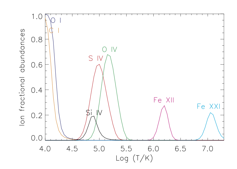
Figure 2.1. Ionization equilibrium balances for some of the optically-thin lines observed by IRIS, obtained using the CHIANTI routine read_ioneq.pro and atomic data included in CHIANTI v.8.
Note
Note that the ionization balances in CHIANTI version 8 and earlier are calculated in low-density (coronal model) approximation. Taking into account the effects of high densities on the ionization equilibrium (in particular the suppression of dielectric recombination) may affect the ionization balances significantly. See an example of the high-density effects on the formation of the IRIS TR lines in Figure 2.2, as studied by Polito et al. 2016, ApJ, 594, 64. See also Nikolic et al, ApJ, 768, 1 ; Young et al. 2018, ApJ, 857, 5 and chapter 3.5.6 of Del Zanna & Mason 2018, LRSP, 15, 5 for more on this topic. See also Sect. 5.1. NB:CHIANTI version 9.0 allows for the exploration of the density sensitivity of some of the satellite lines in a limited wavelength range. Young et al. 2019.
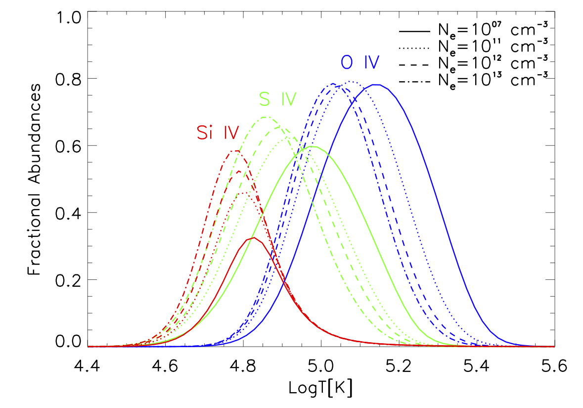
Figure 2.2. Ionization equilibrium balances for the TR lines observed by IRIS calculated taking into account the effect of high densities on the line formation using atomic data from the OPEN-ADAS database. From Polito et al. 2016, ApJ, 594, 64.
2.3. Line intensity and contribution function
In optically-thin conditions, the number of photons in a spectral line observed at a distance d is given by the sum of all the photons emitted by each plasma volume dV along the line-of-sight. Considering a photon of energy \(\frac{hc}{\lambda}\) emitted by spontaneous radiative decay from the energy level j to i, the total emissivity \(\epsilon_\textrm{ji}\) of the j -> i transition will be given by:
where \(A_\textrm{ji}\) is the Einstein coefficient of spontaneous emission of the transition j -> i and \(N(X^\textrm{+z}_\textrm{j})\) is the number density of the the \(X^{+z}\) ion in the excited level j. The Aij value depends on the atomic number of the ion and is usually much larger for allowed transitions, smaller for intercombination transitions and very small for forbidden transitions. The intensity of an optically thin spectral line at wavelength \(\lambda\) is thus given by:
\(N(X^\textrm{+z}_\textrm{j})\) can be expressed as:
where \(\frac{N(X^\textrm{+z}_\textrm{j})}{N(X^\textrm{+z})}\) and \(\frac{N(X^\textrm{+z})}{N(X)}\) represent the relative level and ion populations respectively and \(N_\textrm{e}\) is the plasma number electron density. \(A_\textrm{b}(X)=N(X)/N(H)\) is the abundance of the element X relative to hydrogen and \(N(H)/N_\textrm{e}\) is the hydrogen abundance relative to the free electron density, which in the solar atmosphere is usually taken as ~0.83.
Using the equations above, we can define the contribution function \(G(T,N_\textrm{e},\lambda)\) as:
The contribution function contains all the information on the atomic processes which contribute to give rise to the emission line. Figure 2.3 shows the contribution functions for a set of spectral lines observed by IRIS, which have been calculated using the IDL routine gofnt.pro (see below) and atomic data available in CHIANTI v.8.
-
pro gofnt
Purpose: calculates contribution functions (line intensity per unit emission measure)
Usage:
gofnt,Ion,Wmin,Wmax,Temperature,G,Desc,density=density, lower_levels=lower_levels, upper_levels=upper_levels [+keywords]
Parameters
- Ion: the CHIANTI style name of the ion, i.e., si_4 for SI IV
- Wmin: minimum wavelength (Å) in the wavelength range of interest
- Wmax: maximum wavelength (Å) in the wavelength range of interest
The lower/upper level of the transition can be also specified, in addition with the abundance and ionization equilibrium files. For example, the calling sequence for calculating the contribution function for the Si IV 1402.77Å will be:
gofnt, 'si_4', 1402., 1404., t_si_4_1403, gof_si_4_1403, desc_si_4_1403, dens=dens,
lower_levels=1,upper_levels=2,abund_name=abund_name,ioneq_name=ioneq_name
where one can choose e.g. abund_name=!xuvtop+'/abundance/sun_photospheric_2009_asplund.abund for photospheric abundances from Asplund et al. 2009. The idl routine which_line.pro can be used to find the lower/upper levels of a specific atomic transition given the input wavelength in Angstrom.
-
pro which_line
Usage:
which_line, ionname, wvl,[+keywords]
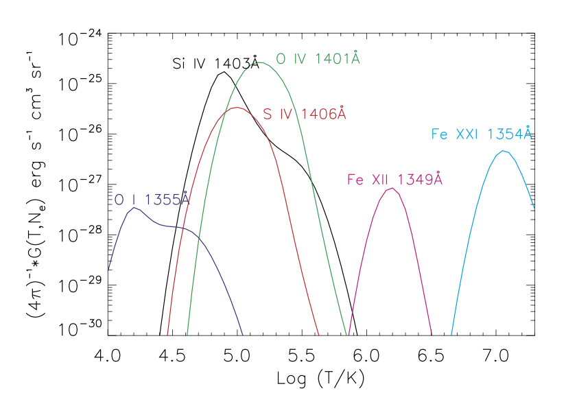
Figure 2.3 Contribution functions (in a log scale) for a set of spectral lines observed by IRIS. Calculated using the CHIANTI routine gofnt.pro , assuming photospheric element abundances from Asplund et al. 2009, ARA&A, 47, 481 and an electron number density Ne of 1011 cm-3 .
The intensity of an emission line can thus be re-written as:
The quantity \(N_\textrm{e} N_\textrm{H} dV = d(\textrm{EM})\) defines the differential emission measure (DEM) of the plasma in the volume dV. The total EM of the plasma is given by integrating over the total emitting volume V:
2.4. Non-equilibrium effects
The spectra of optically-thin lines are often interpreted assuming equilibrium conditions, i.e. the physical conditions of the plasma are time-independent and are described assuming that the particles possess an isotropic, Maxwellian distribution of velocity. Departures from these conditions can occur during highly dynamic phenomena and can lead to non-equilibrium ionization and non-thermal particle distributions. Both effects can be important for plasma diagnostics, as mentioned in Sect. 5.
Non-equilibrium ionization: If the temperature of the plasma changes on a very short timescale, an ion population may be present at much different temperatures than those at which it would normally form in equilibrium. Under non-equilibrium ionization conditions, one needs to solve the set of all time-dependent ionization balance equations to determine the ion populations over time. The intensity of a spectral line can be significantly different in non-equilibrium than in equilibrium ionization (see Figure 2.4). The literature o time-dependent ionization is vast, including earlier work by e.g. Raymond & Dupree 1978, ApJ, 222, 379, Noci at al. 1989, ApJ, 338, 1131, and more recently by e.g. Bradshaw & Mason 2003, A&A, 401, 699, Doyle et al. 2013, A&A, 557, Olluri et al. 2013, ApJ, 767, 43, Martínez-Sykora et al. 2016, ApJ, 871, 46.

Figure 2.4: Contribution functions for Si IV (top) and OIV (bottom) in ionization equilibrium (violet curve) and time-dependent ionization at different times, as marked. From Doyle et al. 2013, A&A, 557, 9.
Non-thermal particle distributions: The assumption of Maxwellian distribution for the electron and ion velocities in a plasma is valid if the energy redistribution through particle collisions takes place on a sufficiently short time scale. In low density and inhomogeneous hot plasma, such as in the outer solar atmosphere, or in the presence of dynamic phenomena such as flares, the timescales for equilibration may be longer. The presence of non-Maxwellian distributions can significantly alter the properties and ionization balance of the plasma (see e.g. Figure 2.5). \(\kappa\) (or generalized Lorentzian) distributions provide a very convenient tool to describe the non-thermal behavior of the particles, as they are characterized by only three independent parameters (n, T, and \(\kappa\)). The KAPPA-package (Dzifčáková et al. 2015, ApJS, 217, 14) provides a collection of atomic data based on the CHIANTI database for non-Maxwellian \(\kappa\)-distributions.
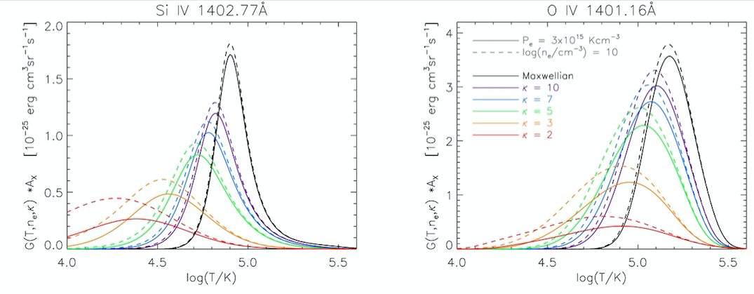
Figure 2.5: Contribution functions for the Si IV 1402.77 Å (left) and OIV 1401.16 Å (right) lines for Maxwellian as non-Maxwellian distributions with different values of \(\kappa\) , as indicated by the legend. From Dudík, et al. 2014, ApJ, 780, 12.