2. IRIS² in SolarSoft
IRIS² is part of IRIS branch in SolarSoft distribution. Since August 2019, SolarSoft (including the associated databases) requires to use wget to be upgraded. If SolarSoft is not installed in your machine or it has not been upgraded since August 5, 2019, then you should follow the instructions given in the SolarSoft Installation web page.
If your computer is running under MacOS and it does not have wget installed, you may find the executable file here.
If you already have SolarSoft and wget installed (after August 2019), then the simplest way to install or upgrade IRIS branch is to run the following command in IDL:
IDL> ssw_upgrade, /iris, /spawn, /wget, /loud
In addition to the IDL IRIS² code, you should install the IRIS² database in your SolarSoft distribution. That requires to have defined an
environment variable called $SSWDB. This variable should point to where all the databases of SolarSoft are stored. A directory called $SSWDB/iris should exist for the proper installation of IRIS² database. You can download or upgrade the IRIS² database, which will be stored or upgraded in $SSWDB/iris/iris2 by using this simple command:
IDL> sswdb_upgrade_wget, 'iris/iris2', /lmsal, /spawn
Finally, you may be interested in to include the IRIS branch, which includes IRIS² code, to the instruments loaded when a SolarSoft session is started. To include them, you should define an environment variable called SSW_INSTR before starting a SolarSoft IDL session. First, you need to know what kind of shell you are using in your system. You can know that by typing:
%echo $SHELL
Once you know what kind of shell you are using (by default) when you start a session on your computer, then you can define the
environment variable SSW_INSTR as follows:
In tcsh or csh:
% setenv SSW_INSTR "iris your_own_list_of_instruments"In bash:
% export SSW_INSTR="iris your_own_list_of_instruments"
Where your_own_list_of_instruments may contain a list of instruments included in your own SolarSoft installation, e.g.: “hinode sot sdo hmi aia soho mdi”.
These commands may be included in the corresponding .tcshrc, .cshrc, or .bashrc files, which will set SSW_INSTR every time a tcsh, csh, or bash session
is started.
The last option will automatically load IRIS (and any other instrument include in SSW_INSTR) at any time an IDL SolarSoft session is started. If you want to load IRIS branch ocassionally – of course, it has been to be installed in your SolarSoft distribution–, then you may execute the following command inside an IDL SolarSoft session:
IDL > ssw_path, /iris
After successfully completing all these steps, then you are ready to use IRIS² in IDL SolarSoft.
2.1. Standalone installation
A minimal distribution of the IRIS branch, including IRIS² code and IRIS² dababase can be found here. You can clone this distribution to your local machine using:
your_prompt> git clone https://gitlab.com/LMSAL_HUB/iris_hub/iris2.git
Then, you can execute the file run_iris2.tcsh.
This script starts a tcsh session. The script
sets the $SSW, $SSWDB, and SSW_INSTR variables, and starts a SolarSoft session with the IRIS branch properly
addressed. Because, these steps are done during the execution of the script, the values of the
enviroment variables $SSW, $SSWDB, and $SSW_INSTR remain local during the session. That means, if they
exist previously in the user’s local machine, then they keep their original values after the session
started by the script is finished.
Thus, you may use:
your_prompt> ./iris2/run_iris2.tcsh
This file has to be executable. Therefore, you can use:
your_prompt> chmod a+x ./iris2/run_iris2.tcsh
If you decide to use this miminal version of IRIS branch as your default option, we suggest you to update both the IRIS² code and the IRIS² database as it is indicated above.
2.2. Inversion of IRIS Mg II h&k lines with iris2
iris2 allows us to recover a model atmosphere and its uncertainties from a IRIS level2 raster file or a list of such files. It is a requirement that the rasters
contain observations of (at least) any of the Mg II h&k lines or the Mg II UV triplet lines between the Mg II h&k lines. That means that for all normal IRIS observations (OBS 36*, 38*, 40*), it should be possible to obtain an inversion. The (minimal) output of iris2 consists of a model atmosphere with the following physical variables and their uncertainties: \(T[kK],\ v_{los}[cms^{-1}],
\ v_{turb}[cms^{-1}],\) and \(n_e[cm^{-3}]\). We will refer to the output structure obtained from iris2 as iris2model.
Once the Mg II h&k lines data in the IRIS level 2 raster file have been found and loaded, iris2 performs the following steps:
the data is cropped in wavelength, so all the data have common sampled wavelengths. We will call these the observed wavelengths; then the data are masked with a 2D binary mask to remove any pixels with the DNs below 0 or that contain NaN values;
the data are calibrated following the process described in Section 5.2 of ITN26;
the data are transformed from a 3D data cube (with dimensions [X,Y, \(\lambda\)]) to a 2D array (with dimensions [X \(\times\) Y, \(\lambda\)]); the
inverted RPs in the IRIS² database are interpolated to the observed wavelengths; iris2 looks for the closest RP in the IRIS² database to the observed profile, determined by the
\(\chi{2}\) (see Eq. 1 in Sainz Dalda et al. 2019) between the observed profile and the RPs in the database; the RMA corresponding to the RP found by iris2 is assigned
to the pixel where the observed profile is located; and the uncertainty from the assigned RMA, the found RP, and the observed profile is calculated as described in Eq. 2 of Sainz Dalda et al. 2019.
By default, iris2 searches the entire IRIS² database, i.e. not taking into account the location where the RPs in the database were observed. The user may
change this behavior with the keyword delta_mu. Thus, the user can constrain the search in the database to RPs located in an interval in \(\mu\) closer to the
\(\mu\) of the observation. That shrinks the number of RPs to compare with the observed profile, which makes the inversion faster. See the considerations about
observations close to the limb noted in Limitations of :math:`IRIS^{2}` inversions.
Another way to accelerate the inversion is to use the PCA decomposition of the observed profiles in the PCA space of the RPs in the IRIS² database. Thus, the iris2 algorithm looks for the closest PCA coefficients of the RPs to the PCA coefficients of the observed profile. The number of eigenvector (and coefficients) considered is 100 by default, since tests have proven that the difference in the RPs found by iris2 using the full profile and the PCA approach is ~0.1% with a gained time of ~40%. This parameter can be changed with the keyword pca. By default, IRIS² does not consider this PCA approach.
Several levels of information can be stored during the inversion. A detailed description of these levels and the variables stored in each level is given in Section 2.4. The level of information is by default 0, but this can be changed using the keyword level.
The output of the code is a structure for a single IRIS Level 2 raster file or an array of structures, if a list of IDL Level 2 raster files was given as an input. We refer to this structure as iris2model.
The structure contains the model atmosphere and the
uncertainties of the variables considered in the model atmosphere. Depending on the level of information given during the inversion, other variables will be
stored in the output structure. See Section 2.4 for a detailed description of the iris2model structure.
2.3. Inversion of a large raster file, a region of interest, or a masked area
Some raster files may be very large in size. That can be a problem in systems with a small memory capacity. In that case, IRIS² has the option to make the inversion of these large raster files in smaller pieces. The keyword in_parts divides, by default, the raster in 3 parts along the scanning direction, i.e., in the direction perpedicular to the slit. If a value larger than zero is given to in_parts, the raster will be split in in_parts portions. IRIS² will return as many output structures iris2model as portions the raster has been split into. Likewise IRIS² will created as many IDL .sav files as portions the raster has been split into. The name of these files will contain an extra text indicating the part with respect to the total of the portions of the raster was split. For instance, iris2model_20160114_230409_3630008076_raster_t000_r00000_part_02_03.sav indicates that the IRIS level 2 raster file iris_l2_20160114_230409_3630008076_raster_t000_r00000.fits was split in 3 parts, with the former file containing the \(2^{nd}\) part of the total of 3.
Other possible scenario may happen when we are interested in just a particular region of the
total area observed by the raster. IRIS² offers two options:sel_roi and my_mask.
The keyword sel_roi allows the user to select as many regions of interest (ROI) as s/he wants to. When this keyword is set to a value different from zero, IRIS² will load the raster and will show a reference image. The user may select a ROI by pressing S in the first corner of the box that will define the box containing the ROI, and a second press on S will store the second corner of the box. The user can enlarge or shrink the reference image by pressing + and - respectively. It is possible to zoom in in the reference image by pressing I to set the first corner of the zoom-in area, and by pressing again I to set the second corner of the area to be zoomed in. A single press on O zooms out to the full view of the reference image. The user may select as many ROIs as s/he is interested in. By pressing Q the user quits the reference image as the inversion of the ROI(s)
starts.
In this case, IRIS² will invert those pixels contained in the ROI that are possible to invert. IRIS² will save as many output structures iris2model as
ROIs have been defined by the user. These output are saved in a IDL .sav file with an extra text in its name that tells us the number of the ROI with respect to the total ROIs selected by the user. For instance, iris2model_20160114_230409_3630008076_raster_t000_r00000_roi_01_02.sav indicates that the user selected 2 ROIs in the IRIS Level 2 files iris_l2_20160114_230409_3630008076_raster_t000_r00000.fits, with the \(1^{st}\) ROI saved in the former file.
On the other hand, if we are interested in inverting an area with a shape more complex
than a simple box (or combination of boxes), the user has the option to give her/his
own binary mask (or an array of them) to IRIS² through the keyword my_mask.
The mask has to have the same size as the observation, the X axis of
the mask defining the direction perpendicular to the IRIS slit. More than one mask may be given by setting
my_mask equal to an array of masks, with the different masks stacked in the \(3^{rd}\) dimension
of that array. Only those pixels with values
equal to 1 in each mask (and in the original mask of the data) will be considered for the inversion .
In this case, the output structure iris2model and the IDL .sav file have
the same size that the original observation, although the inversion has only been done
in the profiles corresponding to the pixels previously mentioned. In this case
the name of the saved files takes the form iris2model_20160114_230409_3630008076_raster_t000_r00000_mymask_01_01.sav.
For all the keywords in_parts, sel_roi and my_mask, IRIS² stores in iris2model the inverted area with respect to the original reference image in the variable mask_extra, and the values needed to define that region in mask_extra_data. Thus, the user can recover at any time the location either of the part or the ROI inverted with respect to the original data. Note that the variable mask_ondata defines the location of all the profiles (pixels in the reference image) susceptible to be inverted in the original raster.
In summary, IRIS² offers three options with different pros and cons:
in_partsdivides the original data in as many parts as the value passed through this keyword (3 by default). It is intended to be used for the inversion of large raster files that may evenutally exceed the memory capacity of the user’s system. The total size of the files after the split is slightly larger than the size of a single file containing the inversion of the full raster. The total execution time is much larger when the raster is split than when it is inverted in a single run.
sel_roiallows the user to select ROIs (boxes) in the observation. Each ROI is inverted as an individual observation. Therefore, the output structureiris2modelcontains the model and uncertainties corresponding to the selected ROI. Hence, the size of the IDL .sav file is smaller than the file corresponding to the original inversion, and the total execution time is shorter as well.
my_maskaccepts a binary mask (or an array of them) with the same size – in the direction along the slit and perpendicular to this one – that the observation. Because of this, the size of theidl2modelstructure and the IDL .sav file is the same that the original observation. The main advantage in this case lies in the execution time, which is shorter than for the original observation, and a better definition of a solar structure of the interest of the user, e.g. a plage region, the penumbra, or umbra, than the one s/he may have with boxes.
Figure 2.1 shows three examples of the masks used in each of the keywords explained above.
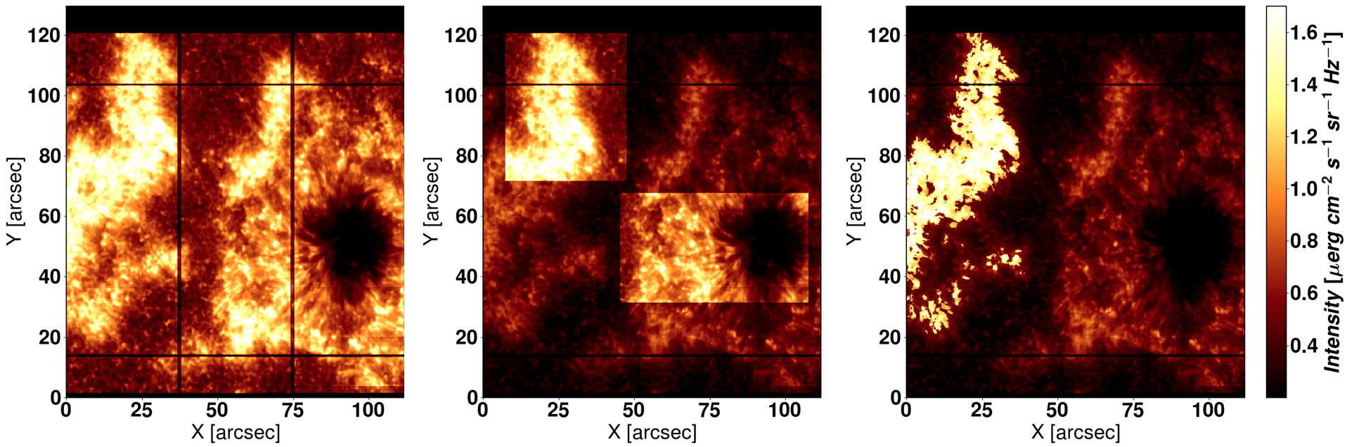
Figure 2.1 Left: The three parts considered with in_parts=1 (default option). Center: The ROIs selected by the user wiht the option
sel_roi. Right: A mask given to IRIS² by the user through the keyword my_mask, considering just the sea-horse-shaped plage.
All these options are only available when a single raster is being inverted.
2.4. The function iris2
-
function iris2, file_irisl2, version_db=version_db, delta_mu=delta_mu, level=level, ...
- PURPOSE:
To recover the model atmosphere (T, vlos, vturb, electron density) from IRIS Mg II h&k lines using \(IRIS^2\) inversion code (Sainz Dalda et al., 2019, ApJL 875 L18).
The code transform the data units to c.g.s units \([erg\ cm^{-2}\ s^{-1}\ sr^{-1}\ Hz^{-1}]\), interpolates the synthetic RPs in the IRIS² database to the observed spectral positions, and looks for the closest inverted RP in that database.
It returns the model atmosphere structure (including the uncertainties) for the IRIS Mg II h&k raster(s), and other information about the inversion depending on the level of information asked for.
- CATEGORY:
Data processing/Inversion
SAMPLE CALLS:
IDL> raster_files = file_search(path_to_IRIS_l2+'/*iris_l2*raster*fits')  ; List of IRIS Level2 raster files
IDL> iris2model = iris2(raster_files) ; Default call: latest |IRIS2| database, considering all RPs (delta_mu=1), level=0, no weights
IDL> iris2model = iris2(raster_files, version_db='v1.0', delta_mu=0.20, level=2)
IDL> iris2model = iris2(raster_files, weights=[1.,1/2.,1.,1/3.], level=1)
- INPUTS:
raster_files: an IRIS Level 2 raster file or a list of these kind of files belonging to the same raster observation, i.e. with the same observation parameters and IRIS OBSID.- OUTPUTS:
iris2model: a structure or an array of structures as large as the list given byraster_files. Depending on thelevel_infovalue, the structure will contain more detailed information about the way the inversion was made. See description inlevelkeyword for more details.- KEYWORDS:
cpu_percentage: A value between 1-100. A percentage of the CPUs used during the inversions. By default, 90% of the CPUs are used.nosave: by default, the iris2structure is saved in the current working directory. Ifnosaveis set (different from 0) nothing is saved.name_save: alternative name of the file where the output is saved. Do not include the directory. The default name is the IRIS Level 2 where ‘iris_l2’ has been changed to ‘iris2model_l2’. If the input was a list of rasters, then ‘raster_xxxxx’ is changed to ‘raster_multi’.dir_save: directory where the output file is saved instead of the current working directory (default).version_db: Currently (20190420) there are 2 version of IRIS² database. The default value is the latest IRIS² database, up to date v2.0, which has ~50,000 RPs/RMAs/RFs, that come from the clustering of 305 observations in 160 RPs per data set. IRIS² database v1.0 has ~15,000 RPs/RMAs/RFs, which come from the clustering of 250 observations in 60 RPs per data set. IRIS² will work faster with IRIS² database v1.0 since the database is smaller, but the results will be more accurata with IRIS² database v2.0. The accepted values are:‘v1.0’: for the version 1.0 of IRIS² database.
‘v2.0’: (default) for the version 2.0 of IRIS² database.
delta_mu: delta in mu value with respect to the mu value of the observation considered during the inversion, e.g. for an observation at mu = 0.73 and delta_mu = 0.2, IRIS² code only considers those RPs coming from observations in the IRIS² database located in 0.53 < mu_in_db < 0.93. If delta_mu=1 (default), then all the RPs in IRIS² database are considered.pca: if it is different than 0, the observed data will be projected on the PCA components of the IRIS2 database. The number of eigenvectors used is the number passed through this keyword if it is larger than 20, otherwise it is 20. This method determine the closest RP in the IRIS2 database to an observed profile calculting the distance between the eigenvalues of the observed profile projected on the PCA components of the IRIS2 database and the eigenvalues of the RPs in the IRIS2 database. See Section 2.2 for more details.weights_windows: a 4-element float variable (e.g., \([w_1, w_2, w_3, w_4] = [1.,1/2.,1.,1/3.]\)) corresponding to the weights in the 4 weighting windows described in Section 1.3.1 and shown in the Figure 1.2. These weighting windows are located around the Mg II k line (\(w_1\)), the Mg II UV lines between the Mg II h&k lines (\(w_2\)), the Mg II h line (\(w_3\)), and finally some spectral positions in the bump located between the Mg II h&k lines, and others in the far red wing of Mg II h line.weights_windowsrequires 4 float values, whether the observed profile has all the spectral ranges just mentioned or not. For instance, an observation with only Mg II k and Mg UV lines will still require a variable like [1.,1/2.,100.,1/3.]. Ifweights_windowsis properly given toiris2, and it is different from zero,iris2will only consider those weights of the spectral ranges observed. In the previous example,iris2would consider \(w_1 = 1.\) and \(w_2 = 1/2.\), and \(w_4 = 1/3.\), since some spectral points between the Mg II k line and the Mg II UV lines belong the weighting window associated the bump. Because in this example the Mg II h line was not observed, then \(w_3 = 100.\) is not considered, but it is mandatory to supply a value for \(w_3\). By default (weights_windows = 0) IRIS² does consider neither weights nor weighting windows. That means,iris2considers all the spectral positions equally by default. For the sake of simplicity,weights_windows = 1is equivalent toweights_windows = [1., 1., 1., 1.]. This is the only exception to the 4-element float input of this keyword.in_parts: divides the original data in in_parts portions. If the value passed is 1, the data are divided in 3 portions (default option). See Section 2.3 for details.sel_roi: when set different than zero, this option allows the user to select as many regions of interest (ROIs) as s/he wishes. See Section 2.3 for details. It accepts a structure as the one given bymask_extra_dataas an input. Thus, the user can use a ROI defined previously for a new inversion. That can be useful when the user is interested in the same ROI in different raster files.my_mask: accepts a binary mask with the same size in the direction along the slit and the perpendicular direction to the former. The pixels in the binary mask with values equals to 1 will be considered to be inverted. Those with values equals to zero will not. See Section 2.3 for details.level: level of information stored in theiris2modelstructure. It has three possible values:- Level 0: Default option. The
iris2modelstructure will contain: input_filename: the raster(s) input filename(s) to be inverted.output_filename: the output filename with theiris2modelstructure.inv_db_fits: FITS file containing the RPs in the IRIS² database.model_db_fits: FITS file containing the Representative Model Atmospheres (RMAs) of IRIS² database.rf_db_fits: FITS files with the response functions (RFs) of the corresponding RMAs-RPs in IRIS² database. This value is used to calculate the uncertainty (see Eq. 2 in Sainz Dalda et al. 2019).nodes_db_fits: FITS files with the positions in optical depth considered during the inversion of the RPs by STiC as nodes. These positions are also used to calculte RFs.ltau: optical depth given as \(log(\tau)\).model: model atmosphere recovered byiris2. It consist of T, vlos, vturb, and electron density.model_dimension_info: information of the dimensions in model. They are: [X [px], Y [px], log(tau), physical_variable]physical_variable: physical variable and units stored in the model: These are: [‘T [k]’, ‘v_los [m/s]’, ‘v_turb [m/s]’, ‘n_e [cm^-3]’]uncertainty: uncertainty of the model, given in the same units that in model.uncertainty_dimension_info: information of the dimensions in uncertainty: These are: [X [px], Y [px], log(tau), uncertainty_in_physical_variable]uncertainty_variable: uncertainty for each variable in the model: These are: [‘unc_T [k]’, ‘unc_v_los [m/s]’, ‘unc_v_turb [m/s]’, ‘unc_n_e [cm^-3]chi2: \(\chi^{2}\) map calculated as Eq. 1 in Sainz Dalda et al. 2019.weighting_windows_01: 0/1 binary mask in the observed wavelengths given inwl, where 1 represents the spectral position considered in the calculation of closest RP in the IRIS² database, \(\chi^2\), and \(\sigma_p\). By default, all the observed spectral positions are considered, therefore, the default values ofweighting_windows_01are all 1s. Ifweigthsis a 4-value variable, and different from zero, the values equals to 1 are given to 4 predefined weighting windows. SeeUnderstanding the quality of the |IRIS2| resultsfor more details.weights_in_windows: the weights \(w_i\) considered at an observed spectral position inwl. By default, all the weigths are 1s. The values are considered in the 4 pre-defined weighting windows. SeeUnderstanding the quality of the |IRIS2| resultsfor more details.pca_components: the number of PCA coefficients given by the keywordpca. If it is not set (default), then it equals -1.header: header corresponding to the original IRIS_lev2 raster file.mu: mu of the observed datadelta_mu_db: interval in mu (cos(theta), being theta the heliocentric angle) used to look for RPs in the IRIS² database.level_info: level of information demanded vialevelkeyword: 0 (default), 1 or 2.qc_flag: quality control flag:0: No raster file, nothing is inverted
1: inversion completed succesfully
-1: Something went wrong: none data were inverted, nothing was saved.
- Level 1: the information obtained with Level 0 plus:
wl: original wavelengths sampled in the IRIS observations used during the IRIS² inversion.nodes_positions: a structure with the values of the nodes used to calculated the RFs for T, v_los, v_turb, and n_e.nodes_values_in_ltau: a structure with the values of the nodes in optical depth (log(tau)) used to calculated the RFs for \(T, v_{los}, v_{turb}\), and \(n_e\).flag_mask: a 4-value variable indicating what mask option has been used with a value 1. The meaning of the positions is \([default, sel\_roi, in\_parts, my\_mask]\). For instance,flag_mask= [0,0,1,0] indicates that the optionin_partswas used during the inversion.iris_cal: datacube with the original data calibrated in c.g.s units \([erg\ cm^{-2}\ s^{-1}\ sr^{-1}\ Hz^{-1}]\) in the wavelengths inwl.units_iris_cal: \([erg\ cm^{-2}\ s^{-1}\ sr^{-1}\ Hz^{-1}]\)iris2_inv: datacube with the RPs in the IRIS² database that matches best the observed profiles. It is interpolated to the observed wavelengths inwl.units_iris2_inv: \([erg\ cm^{-2}\ s^{-1}\ sr^{-1}\ Hz^{-1}]\)weight2noise: a 3D variable with the values or \(w_i/\sigma_i\) used to calculate \(\chi^2\) and the uncertainties \(\sigma_p\) (seeUnderstanding the quality of the |IRIS2| results). Its dimensions are [X, Y, \(\lambda\)].
- Level 2: the information obtained with Level 1 plus:
mask_ondata: a binary mask considering those pixels in the original data susceptible to be inverted.mask_extra: by default, this mask is the one defined inmask_ondata. Ifsel_roi,in_partsormy_maskare given, the mask inmask_extrais the multiplication ofmask_ondataand the mask defined by these keywords. See Section 2.3 for details.mask_extra: a structure containing the coordinates of the left bottom corner \((xb,yb)\), the width \((nxb)\), and the heigh \((nyb)\) of the mask defined inmask_extra.ima_ref: a reference image used to define the boxes by the user with the optionsel_roi. This image corresponds to the integrated intesity over all the spectral wavelengths considered in the observation and defined inwl.ima_ref_mask: the reference image given inima_refwith the area defined by the mask given bysel_roi,in_partsormy_maskhighlighted.n_w_mask: number of pixels in the mask with value 1 inmask_extra. Note that for the default case, becausemask_ondataandmask_extraare the identical, this number is the number of pixels in the mask with value 1 inmask_ondtaas well.n_rp_db_used: the number of RPs in the IRIS² database considered during the inversion. This number may be different to the total number of the RPs in the IRIS² database if we consider the optiondelt_mu.map_index_db: a map with the index of the RPs in the IRIS² database that best matches the observed profile in that pixel.map_mu_db: a map with the mu value corresponding to the RPs in the IRIS² database that best matches the observed profile in that pixel.factor: structure containing all the information used for the calibration.partial_execution_time: execution time taken for the inversion of an input raster.total_execution_time: execution time taken for the inversion of all input rasters.threads_used: CPUs or threads used during the inversion.batch_size: batch size used to split the observed data during the inversion.
- Level 0: Default option. The
2.4.1. IRIS² Tutorial Videos: inverting IRIS Mg h&k lines with iris2
The following videos show how to invert IRIS Mg II h&k data using iris2:
Starting
iris2:Understanding
iris2and its output:Inverting several IRIS Mg II h&k data sets from the same observation (OBSID) with
iris2:Understanding the output when inverting IRIS Mg II h&k data sets from the same observation (OBSID) with
iris2:
2.5. Inspecting the IRIS² model atmosphere (and beyond)
We have developed a visualization tool to facilitate the interpretation of the results obtained with iris2. This tool is called show_iris2model.
The behavior of this function may be different depending on the level of information of the iris2 output structure (see level in Section 2.4). Thus, if iris2model.level_info is 0, then the visualization tool will not be able to display the calibrated data and the inverted RPs, since these variables are not available in the iris2model output structure when level_info is 0.
The simplest way to inspect the iris2model structure is by calling show_iris2model function as:
IDL> sel = show_iris2model(iris2model)
show_iris2model will show two or three windows, depending on the level of information of the iris2model output structure. These windows are:
IRIS2 3D Model Inspector: This window will be always able to display the model atmosphere provided by
iris2. However, it may show other variables or other images that have exactly the same size in X and Y that the model atmosphere has.IRIS2 Model Atmosphere: This model will always show the model atmosphere in the position where the mouse is located on the image displayed in the IRIS2 3D Model Inspector window, even when the latter is not showing the model atmosphere.
IRIS2 Fit (only available for
level_infoequals 1 or 2): It shows the calibrated observed data (in dashed line) and the inverted RP corresponding to the position where the mouse is located in the IRIS2 3D Model Inspector window. The inverted RP profile that IRIS² found as the one that matches the observed profile best is overplotted with a thick line. The X axis is given in the observed wavelengths, while the Y axis gives the Intensity in units of \([erg\ cm^{-2}\ s^{-1}\ sr^{-1}\ Hz^{-1}]\).
Warning
Once the visualization tool has started, DO NOT CLICK the mouse on any window except the one running the IDL session. The control of the visualization is taken from the IDL session via keystrokes associated to some actions. When the control is in the IDL session terminal, the cursor character will be a block character like this ▋ (see Figure 2.2). If the control command is not in the IDL session terminal, then the block character is empty (see Figure 2.7). When the control is not in the IDL session terminal a keystroke will have a none effect in the behavior of the visualization, although moving the mouse over the displayed image will still update the information shown in the plots and the labels. You get the control back to the IDL session by clicking in the window (terminal) running IDL.
When a new window is created, for instance, when the size of the displayed image is enlarged or the IRIS2 Fit window is shown, the IDL windows client (e.g. XQuartz) may put the focus of the mouse on those windows. To avoid that, we suggest you to change the preferences of your IDL windows client. For instance, in Mac OSX, after clicking in the Preferences bottom, a window called X11 Preferences will appear. Then, after clicking in the tab Windows, you should keep the option Focus On New Windows unselected.
Figure 2.2 shows these three windows, and the IDL session having the control (full block cursor), as they are usually displayed on the screen.
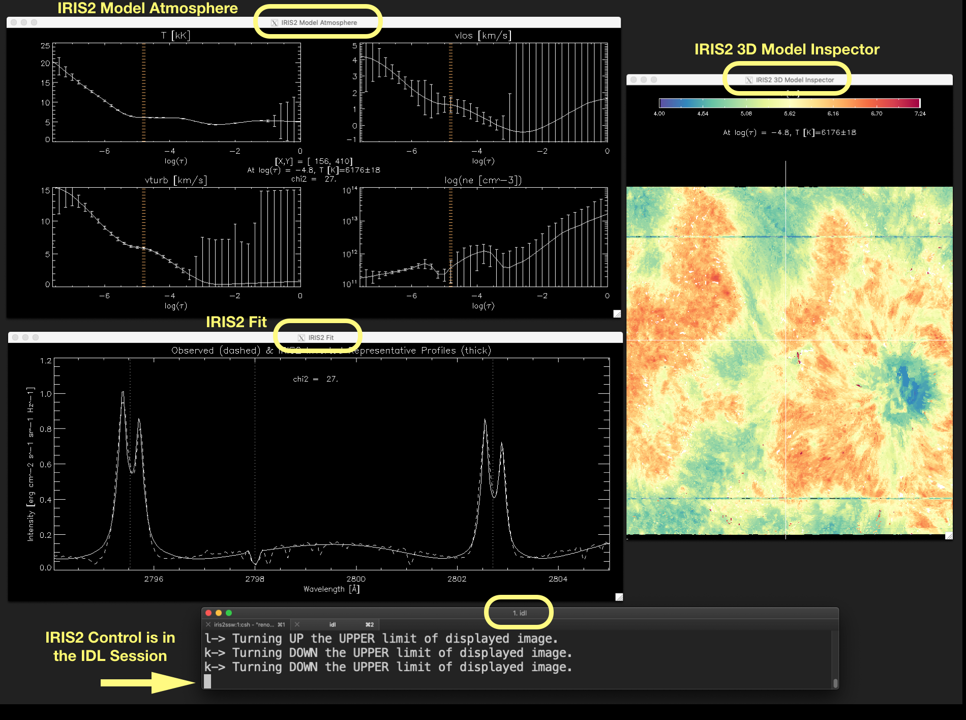
Figure 2.2 Associated windows to show_iris2model with level_info equals 1 or 2, and the IDL session terminal.
The full block character (pointed out by the arrow) indicates that IRIS² control is in the IDL session. Click
on the image to enlarge it.
Figure 2.3 shows the shortcuts of show_iris2model. These shortcuts facilitate the analyze and visualization of
the structure iris2model obtained with iris2. Again, these shortcuts have an effect on show_iris2model as far as the
control is in the IDL session (see Figure 2.2). Otherwise, any keystroke will not have any effect on show_iris2model.

Figure 2.3 Shortcuts for show_iris2model.
2.5.1. The IRIS2 3D Model Inspector window
As we have already mentioned, this window will be always able to display the model atmosphere provided by iris2. However, it can be used to show other images as well. An Auxiliary image can be passed with the keyword aux_image. If the size of the auxiliary image is not exactly the same as the IRIS² model atmosphere, the code will crash. It is highly convenient to give as an auxiliary image an
image co-aligned with and that has the same scale as the inverted data.
The user can change the atmosphere model variable shown in this window by pressing V. Thus, pressing V again and again, it will sequentially display the variables in the cycle \(T[kK] \rightarrow v_{los}[kms^{-1}] \rightarrow v_{turb}[kms^{-1}] \rightarrow log(n_e[cm^{-3}]) \rightarrow T[kK]\).
The window can be enlarged or shrunk by 10% of the current size by pressing + or - respectively. A specific zoom can be passed through the keyword zoom. If zoom is just a number, the same zoom factor will be applied to both the X and Y axes. If zoom is a 2-value variable, the first value (zoom[0]) will be applied to X axis, and the second value (zoom[1]) to Y axis. In addition, the image scale can be changed to arcsec/px through the keyword arcsec. If arcsec differs from 0, the image scale will be divided by the value of arcsec and thus the image size enlarged by the same factor. Thus, for instance, if arcsec is 3, the image will be enlarged by a factor 3, keeping the same aspect ratio as the original image, and the displayed image has a scale image of 1”/3px.
Pressing Z or X will display either the previous or the next image in the model data cube. In this way, the user can inspect the model atmosphere as a function of the optical depth (given as \(log(\tau)\)) by pressing these two letters, going up in the solar atmosphere (towards the transition region) by pressing Z, or downwards (towards the photosphere) by pressing X. When this is done, the displayed image can be poorly contrasted due to the change in the range of values displayed. To improve the visibility of the image, the user can change the upper and lower limits of the displayed image by pressing H or J to decrease or increase the lower limit, and K or L to decrease or increase the upper limit.
The position of the mouse is marked by a crosshair over the image. Do not click on the image, since that would send the control to the IRIS2 3D Model Inspector window, thereby losing the control of the window that includes the IDL command
line. The user can store as many selected positions as she/he wishes by pressing S. The selected positions are returned in the output structure returned by show_iris2model. The [X,Y] position of the mouse is shown and updated in the IRIS2 Model Atmosphere window at all the time the mouse is on the image displayed in IRIS2 3D Model Inspector window.
The name of the physical variable is shown in the colorbar. Below it, the value of that variable and its uncertainty at the current optical depth in the atmosphere datacube is also displayed.
When the user changes the upper or the lower limit of the image, the values in the colorbar change dynamically. For \(v_{los}\), the incremental change is symmetrical by default. Thus, the middle color of the color table (grey by default) corresponds to
the zero value. This behavior can be changed with the keyword asymmetric_vlos.
Figure 2.4 shows some of these elements enclosed in yellow or black (the mouse position).
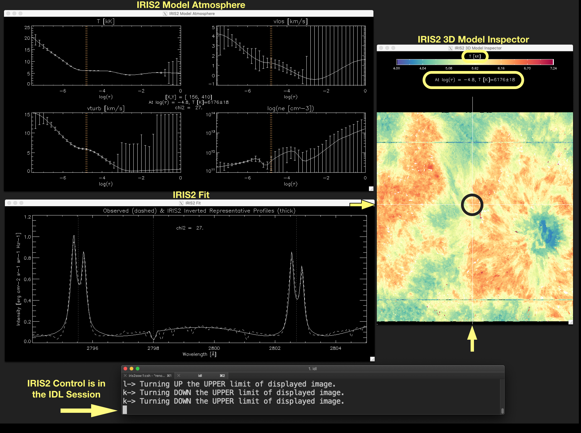
Figure 2.4 The yellow arrows point out the position of the vertical and horizontal lines of the crosshair that marks the position of the mouse (enclosed in a black circle for a better visualization). The displayed variable is indicated above the colorbar. The value of that variable and its uncertainties in the current position of the mouse is shown below the colorbar. Click on the image to enlarge it.
2.5.2. The IRIS2 Model Atmosphere window
- This window shows the atmosphere model and uncertainties provided by IRIS2 along the optical depth (given as \(log(\tau)\)). Thus, from upper left corner, in clockwise direction, \(T[kK], v_{los}[kms^{-1}], v_{turb}[kms^{-1}]\)
and \(log(n_e[cm^{-3}])\) is given for the location indicated by the mouse position in the IRIS2 3D Model Inspector window.
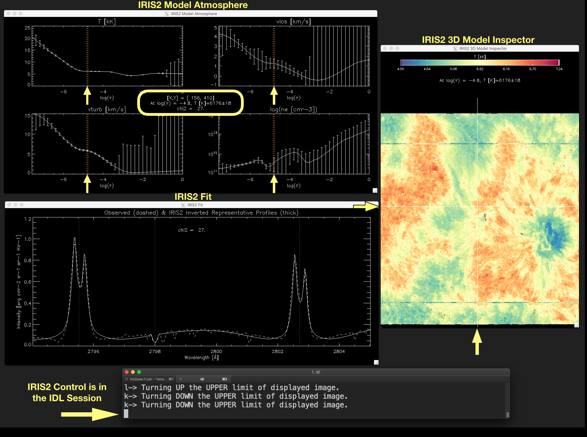
Figure 2.5 The plots in the IRIS2 Model Atmosphere window show the atmosphere model variables \(T[kK], v_{los}[kms^{-1}], v_{turb}[kms^{-1}]\) and \(log(n_e[cm^{-3}])\) at the optical depth indicated by a vertical line in the plots (marked by the arrows) and in the label in the middle of the window. The current position of the mouse marked by the crosshair in the IRIS2 3D Model Inspector window (see the yellow arrows) and the quality of the fit between the observed data and the inverted RP (\(\chi^{2}\)) are also given in the label located in the middle of the window. Click on the image to enlarge it.
A vertical line indicates the optical depth corresponding to the current position in the model atmosphere datacube. This line is updated at any time the user runs through the optical depth in any variable of the model atmosphere by pressing Z or X.
A label in the middle of this window tells us the current position of the mouse on the displayed image ([X,Y]), the value of the atmosphere variable at the current optical depth and its uncertainty at that position – even when the displayed image is not the model atmosphere –, and the quality of the fit between the observed profile and the inverted RP given by \(\chi^{2}\). These elements are marked in yellow in Figure 2.5.
2.5.3. The IRIS2 Fit window
This window will be available for iris2model structure with level_info equals 1 or 2. It may be open and activated by the
keyword show_fit or by pressing F at any time. Pressing F when the window is activated will close it.
This window shows the observed profile (dashed line) and the inverted RP (thick line) found by IRIS² for the position where the
mouse is on the display image. The quality of the fit (\(\chi^{2}\)) is also shown in a label. These elements can be
identified in Figure 2.6.
In addition, if the user presses M and no auxiliary image has been given, the IRIS2 3D Model Inspector window will show the calibrated data cube. That allows the user to inspect the original (calibrated) data, and move through the sampled wavelengths (the 3rd dimension of this data cube) as we did with the model atmosphere, that is, by pressing Z or X. When that is done, a vertical line in the plot shown in this window will mark the position in wavelength used to display a monochromatic image in the IRIS2 3D Model Inspector window. Note that the first position in wavelength often has an intensity that is rather low. Again, the threshold of the displayed image can be changed by pressing H or J for the lower limit, and K or L for the upper
limit. If the user presses M repeatedly, the displayed image will toggle between the loaded model atmosphere variable and the monochromatic image. This allows us to inspect interested areas or features from the observations and to know the thermodynamics of them in an easy and simple way. A reminder: The model atmosphere variable can be changed by pressing V when the model atmosphere is displayed in the IRIS2 3D Model Inspector window.
If an auxiliary image has been given, IRIS2 Fit window will still show the observed profiles and the inverted RP, but as the displayed image is either the auxiliary image or the model atmosphere, pressing Z or X will force the code to run through the 3rd dimension of the model atmosphere. Therefore, no vertical line will be displayed in the plot of the IRIS2 Fit window, but it will be shown in the plots of the IRIS2 Model Inspector window.

Figure 2.6 Fit between the observed calibrated profile (dashed line) and the inverted RP profile (thick line). A monochromatic image created from the calibrated data in the wavelength marked by a vertical line in the plot of the window IRIS2 Model Atmosphere window (yellow arrow) is displayed in the IRIS2 3D Model Inspector window.
2.5.4. The \(\chi^2\)-map, map_index_db, and map_mu_db maps
The \(\chi^2\)-map is available in all iris2model structures. However, the map_index_db and map_mu_db are only
available in iris2model structure with level_info equals 2. Because these maps are part of the iris2model structure they can be displayed easily by using the keywords show_chi2, show_index, and show_mu. If any of these keywords is given, the possibility of showing the calibrated data in the IRIS2 3D Model inspector window is overridden. Therefore, the displayed image in the latter window will toggle between the model atmosphere and the map shown by the keyword given.
These maps are considered internally as an auxiliary image. Hence, the behavior of show_iris2model is the same as when an auxiliary image is given.
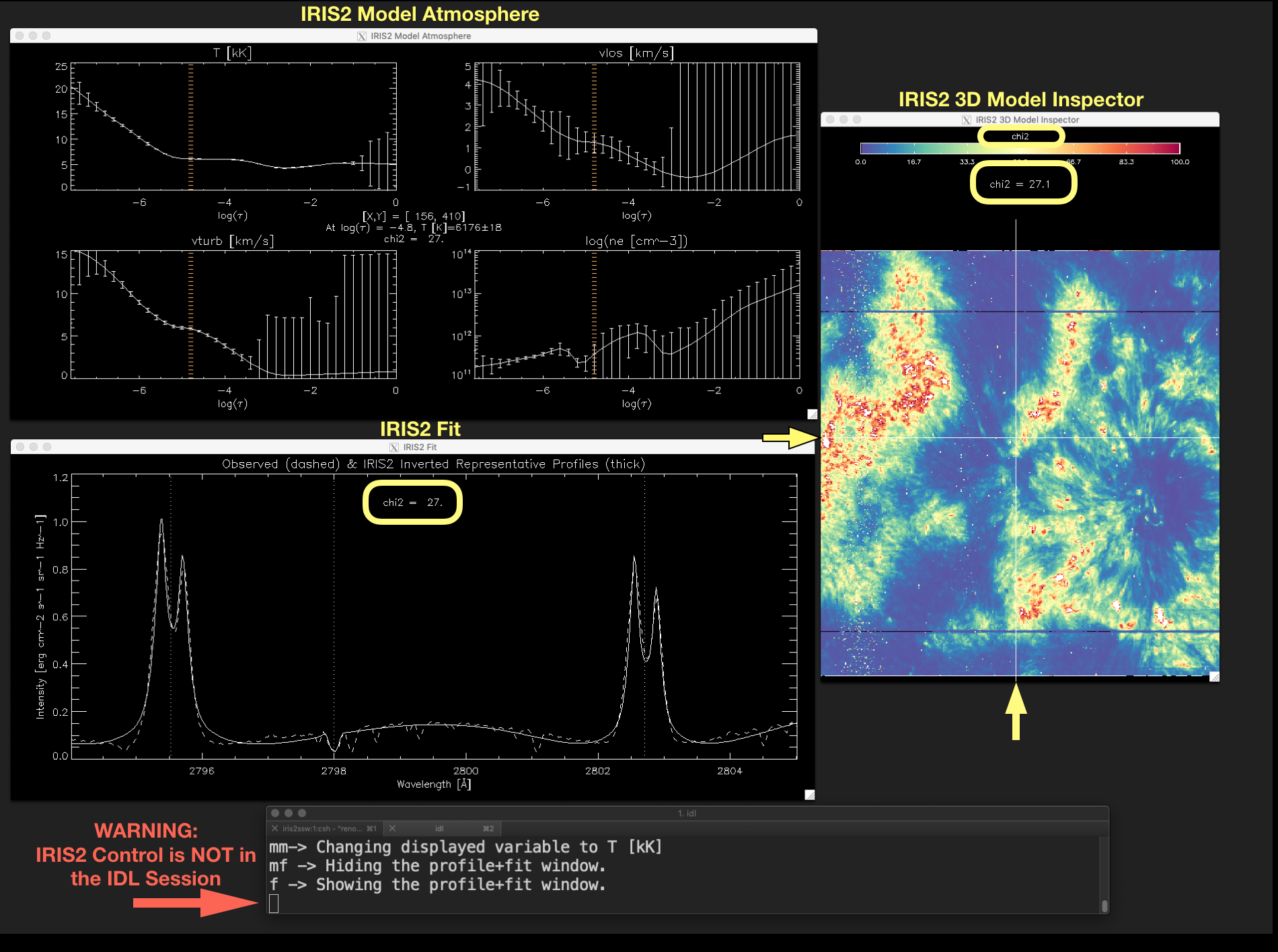
Figure 2.7 \(\chi^{2}\)-map can be shown using the keyword show_chi2. Similarly, a map showing the index of the inverted RPs in
the IRIS² database (map_index_db) and a map showing the \(\mu\) value of the inverted RPs (map_mu_db) can be
displayed using the keywords show_index and show_mu respectively. Notice that in this figure the cursor character in
the IDL session is an empty block character (marked by the red arrow), which indicates the iris2 control is not in the IDL session.
Therefore, any keystroke will not have any effect in show_iris2model. To recover the keystroke control the user must click
with the mouse on the terminal running the IDL session.
2.6. The function show_iris2model
-
function show_iris2model, iris2model, raster_sel=raster_sel, aux_ima=aux_ima...
- NAME:
show_iris2model
- PURPOSE:
To display a model atmosphere (T, vlos, vturb, electron density) recovered from IRIS Mg II h&k lines using IRIS² - or just IRIS2 - inversion code (Sainz Dalda et al., ApJL 875 L18 (2019)). To recover the IRIS² model atmosphere structures see
iris2function.In addition to displaying the model atmosphere, depending of the information level in the recovered IRIS2 model atmosphere structure, this function is able to display the observed and fit profiles, the chi2 map, the index map, and the original data cube.
The function returns a structure which contains information of the points selected by the user.
- CATEGORY:
Visualization. Data analysis.
SAMPLE CALLS:
IDL> sel = show_iris2model(iris2model)
IDL> sel = show_iris2model(iris2model, raster_sel=[1,3], show_fit=1)
- INPUTS:
iris2modelstructure obtained withiris2. Depending of the information contained in this structure the behavior of show_iris2model may be different.- OUTPUT:
By default, if none point has been stored, the output is a structure containing the information about the model atmosphere, uncertainty and other values of the point where the mouse is located. If a position(s) is(are) has(have) been stored by the user pressing “S”, the output is a structure with the position(s) as it is in the displayed image, in the original data, the filenames of the data, and other information for the selected points. Depending on the level of information or
iris2modelstructure the output is:- For
level_infoequals 0: x_display: the X value of the selected point in the displayed image coordinates.y_display: the Y value of the selected point in the displayed image coordinates.x_in_raster: the X value of the selected point in the original data coordinates.y_in_raster: the Y value of the selected point in the original data coordinates.model_xy: the model atmosphere in the selected point.uncertainty_xy: the uncertainty of the model atmosphere in the selected point.ltau: optical depth in log(tau) where the model atmosphere is sampled.chi2_xy: the chi2 of the fit between the observed profile and the inverted RP in the selected point.mu_obs: mu value of the observation.raster_index_xy: the number of the raster for the selected point.raster_filename_xy: the file name of the raster for the selected point.all_rasters_filenames: all the file name rasters considered to buildiris2model, i.e. during the inversion.selected_rasters: the number of the raster(s) selected through the keyword raster_sel.
- For
level_infoequals 1, the variables in the output structure are those in the output forlevel_infoequals 0 plus: iris_cal_xy: the calibrated observed profile in the selected point.iris2_inv_xy: the inverted RP in the selected point.wl: wavelength in Angstrom whereiris_cal_xywas observed and inv_iris2_xy was interpolated.
- For
level_infoequals 2, the variables in the output structure are those in the output forlevel_infoequals 1 plus: index_db_xy: index of the inverted RP in the IRIS² database for the selected point.mu_db_xy: mu value of the inverted RP in the IRIS² database for the selected point.
- For
- KEYWORDS:
show_chi2: it displays the chi2-map.show_index: iflevel_infoin theiris2modelstructure is 2, it displays a map showing the index of the representative profile (RP) used in the IRIS² database during the inversion. Thus, the user can know what RP and from what observation in the database it comes from.show_mu: iflevel_infoin theiris2modelstructure is 2, it displays a map of the mu position of the RP in the IRIS² database used for the inversion.show_fit: iflevel_infoin theiris2modelstructure is 1 or 2, a new window will show the the observed (dashed) and fit profiles (thick), with the chi2 information.put_threshold: sets a threshold for the variables showed.color_index: sets the colortable used to display the data, e.g. color_index = 3 is equivalent toloadct, 3command in IDL. The IRIS² model atmosphere variables have their own default colortables.zoom: If zoom is just a number, the data to be displayed are zoom in/out by a factor of zoom, in both axes (X and Y). If zoom is a tuple, the data to be displayed are zoom in/out by a factor zoom[0] in X axis, and by a factor zoom[1] in Y axis.arcsec: If it equals 1, the data are zoom to the plate scale, i.e. arcsec/px. Thus, if an observation covers an area of 120”x110”, the data are displayed as 120x110 px^2. Because that size may be a small image, if arcsec is a number > 1, it enlarges the data by that factor, e.g. arcsec=3 displays an image of 360x330px^2.raster_sel: List of numbers of the rasters in theiris2modelstructure to be displayed, e.g. raster_sel=[0,3,5] will show the corresponding rasters in theiris2modelstructure. The position of a selected point is returned both relative to the displayed image and to the original raster.
- COMMANDS:
Several commands are encoded in some letters (case-insensitive). This a list of letters and commands and a description of their actions:
To display the description of these commands:
?-> Shows the help information.
Moving along the 3rd dimension in the model atmosphere (optical depth) or the original calibrated data (spectral information). A vertical line pointing out the current position is displayed in the optical depth in the model variables plots or in the spectral position in the profile plots. It changes as:
Z-> Moves back along the 3rd dimension of the data cube.X-> Moves forward along 3rd dimension of the data cube.
Toggles between the model atmosphere and the original (calibrated) data, only if
level_infois 2:M-> Toggles between the model atmosphere and the calibrated data cube or an auxiliary image.
Changes between the variables in the model atmosphere:
V-> Changes the variable displayed following this order: \(T[kK] \rightarrow v_{los}[kms^{-1}] \rightarrow v_{turb}[kms^{-1}] \rightarrow log(n_e[cm^{-3}]) \rightarrow T[kK]\) …
Changing the threshold of the image displayed (not of the values in the data):
H-> Turns DOWN the LOWER limit of displayed image.J-> Turns UP the LOWER limit of displayed image.L-> Turns UP the UPPER limit of displayed image.K-> Turns DOWN the UPPER limit of displayed image.R-> Resets the lower and upper limits of the displayed image.
Activate/Deactivate the profile+fit window:
F-> Shows/Hides the profile+fit window (IRI2 Fit window).
Storing the position and other information:
S-> Stores the position, the corresponding values of model atmosphere and uncertainty in that position and other values depending on thelevel_infoin theiris2modelstructure. The position is stored as it is displayed in the image (in the original scale of the data, i.e. without taking into account the zoom) and as it is in the original raster.
Changing the size of the displayed image:
+/=-> Makes the displayed image 10% larger.--> Makes the displayed image 10% smaller.a-> Changes the displayed image to 1px/arcsec scale.
Zooming in and out:
I: the \(1^{st}\) press stores the \(1^{st}\) corner of the box to be zoomed in. The \(2^{nd}\) press stores the \(2^{nd}\) corner of the box to be zoomed in.O: zooms out to the original data.
Quit show_iris2model:
Q-> Quits show_iris2model.
2.6.1. IRIS² Tutorial Videos: inspecting the inversion results with show_iris2model
The following videos show how to visualize the model atmosphere, uncertainty, and other variables contained in iris2model structure as
a result of the inversion of IRIS Mg II h&k with IRIS²:
Starting
show_iris2model:Moving along the optical depth in the model atmosphere data cube:
Changing the size of the displayed image, and showing other variables of the model atmosphere and the original calibrated data:
Showing the original calibrated profiles and the inverted RP.
Storing selected positions:
Showing multiple inverted raster files corresponding to the same observation (same OBSID):
Storing selected positions from multiple inverted raster files corresponding to the same observation (same OBSID):
Showing other images stored in
iris2model: