1. IRIS²: IRIS Inversion based on Representative profiles Inverted by STiC
IRIS Inversion based on Representative profiles Inverted by STiC or \(IRIS^2\) is an inversion code (IC) devoted to recovering the thermodynamics of the chromosphere and high photosphere using IRIS observations of the Mg II h&k and Mg II triplet lines, all located in the near ultra-violet.
A Representative Profile (RP) is the averaged profile of a cluster of profiles sharing the same shape as a function of wavelength. The RPs of a data set are the averaged profiles obtained from clustering the data set using the k-means clustering method. The shape of a profile is the distribution of the observed intensity with respect to the wavelength. The intensity and shape of a profile encodes information about the interaction between the radiation field and the matter in the atmosphere from which the radiation originates. Locations with similar physical conditions will share profiles of similar shape; a region in the atmosphere with similar thermodynamic conditions is therefore associated with a certain RP - or just a few RPs. This forms the conceptual foundation upon which \(IRIS^{2}\) is based.
Given an observed profile the \(IRIS^{2}\) algorithm will search for the most similar inverted RP in a database built up of inverted RPs, which were derived from observations. These inverted RPs come from IRIS Mg II h&k observations of different solar features with different observational properties (e.g. observing mode, exposure time, spatial sampling, or position on the solar disk). Each inverted RP has an associated Representative Model Atmosphere (RMA), which is the model atmosphere derived by the STiC (de la Cruz Rodríguez et al 2019) inversion code of that observed RP.
This manual shows how to recover (and display) a model atmosphere along the optical depth (\(log(\tau)\)) using \(IRIS^{2}\) in IDL SolarSoft from the IRIS Mg II h&k lines. A more detailed description of \(IRIS^{2}\) may be found in Sainz Dalda et al. 2019.
1.1. Quick start to invert IRIS Mg II h&k lines with IRIS²
To invert IRIS Mg II h&k lines with \(IRIS^{2}\) is very easy. However, it is important to know what we are doing when we use it. This manual explains in detail all the aspects needed to understand how \(IRIS^{2}\) works, its limitations, its options, its output, and the visualization tool to analyze its results. We encourage you read this document to get a better understanding of \(IRIS^{2}\) and the concepts around it. The following lines show how easy it is to obtain a stratified-in-depth model atmosphere and its uncertainties of an IRIS Mg II h&k with \(IRIS^{2}\) in IDL SolarSoft:
IDL> filename = 'iris_l2_20160114_230409_3630008076_raster_t000_r00000.fits'
IDL> iris2model = iris2(filename)
IDL> sel = show_iris2model(iris2model)
If you have an updated SolarSoft distribution, including IRIS branch and IRIS database, these 3 lines are all you need to start analyzing the thermodynamics in the high photosphere and the chromosphere observed with IRIS Mg II h&k lines.
In the following sections you will get all the information you need to obtain the best from \(IRIS^{2}\).
1.2. Limitations of IRIS² inversions
As in any other inversion code (IC), \(IRIS^{2}\) has its limitations. We can identify 3 different kinds of limitations: those due to the \(IRIS^{2}\) method; those that come from the underlying inversion engine STiC; and those caused by the intrensic properties of the Mg II h& k lines. We summarize these limitations as follows:
Limitations due to \(IRIS^{2}\):
\(IRIS^{2}\) is an IC designed for working on any solar feature as observed by the IRIS Mg II h&k lines. We have decided to invert all the RPs in the \(IRIS^{2}\) database using the same inversion setup. This setup consists of 2 cycles: In the 1st cycle using 7 nodes in temperature \(T\), and 3 nodes both in line of sight velocity \(v_{los}\) and turbulent velocity \(v_{turb}\). The 2nd cycle uses 11 nodes in \(T\), and 4 nodes in both \(v_{los}\) and \(v_{turb}\). This setup is good enough for a large variety of profiles, though not for all the profiles; e.g. profiles with extreme line widths such as observed in X-class flares, and UV bursts or explosive events. While we are working to improve \(IRIS^{2}\) in upcoming versions, the current version is not able to fit this kind of profiles. \(IRIS^{2}\) can also have some difficulties with other profiles shapes that superficially appear easy to invert (e.g. plage profiles). Therefore, it is always a good working habit to verify the quality of the fit between the observed and the inverted profiles found by \(IRIS^{2}\), or for that matter any other IC. This check can be done very easily with
show_iris2model, the visualization tool developed for \(IRIS^{2}\) (see Section 2.5).The numbers of RPs per dataset are 60 and 160 for the \(IRIS^{2}\) databases v1.0 and v2.0 respectively. For the \(IRIS^{2}\) database v1.0, the number of RPs is not sufficient to give an accurate representation for some datasets. The reason the number of RPs is limited to 60 is due to hardware constraints during the time we built the \(IRIS^{2}\) database v1.0 (the number of cores in the server at LMSAL was only 120 at the time). We therefore decided to keep that low number of RPs as a good representation for all the datasets. When the IRIS team acquired a server with a larger number of cores the total of RPs was increased to 160 RPs per dataset. This larger number of RPs allows a very good representation of the profiles in most of the datasets in the \(IRIS^{2}\) database. The following video shows the normalized inertia (within-cluster sum-of-squared errors) with respect to the number of RPs for the data sets in \(IRIS^{2}\) database v1.0. In most of the cases, the inertia does not improve significantly for a number of RPs above 160. Moreover, this happens independently of the number of profiles clustered in the dataset, or the exposure time, i.e. the noise. Thus, using 160 RPs per data set is good enough to represent the data sets considered in the \(IRIS^{2}\), independently of the noise amplitude.
Although we have tried to build a database with a homogenous distribution of observed solar features on the solar disk (i.e. in \(\mu\)), the \(IRIS^{2}\) database is not as homogeneous as we would like. Thus, a solar feature, e.g. a coronal hole, may have been mostly observed in locations with 0.6 < \(\mu\) < 1.0. The inversion utility built in IDL to use \(IRIS^{2}\) on IRIS Mg II h&k data, named
iris2, has an option to consider all the RPs in its database (the default), or a smaller subset of RPs constrained to an interval of observations in the \(IRIS^{2}\) database with similar \(\mu\). New datasets in more diverse locations have been included in the \(IRIS^{2}\) database v2.0 as compared to v1.0. We will include more data sets in the coming versions. It is clear that the larger the variety of solar features observed in different locations included in the \(IRIS^{2}\) database the better the results provided by \(IRIS^{2}\) will be. See other important considerations about observations close to the limb in Limitations due to the observed lines.
STiC is capable of inverting the Stokes profiles (I, Q, U, and V) from several atoms in non-local thermodynamical equilibrium (non-LTE), taking into account partial redistribution effects (PRD), in angle and frequency, of scattered photons. \(IRIS^{2}\) only considers intensity profiles (Stokes I) since the IRIS Mg II h&k observations do not have polarimetric information. In the current version (\(IRIS^{2}\) v2.0), only Mg II h&k and the two lines of the Mg II UV triplet located between the k and h lines are considered. Future versions will include photospheric lines.
Limitation due to STiC:
STiC works under the 1.5D approximation: This means that a plane-parallel geometry is assumed when solving the equations of statistical equilibrium, on a column-by-column basis. Once the atomic population densities are known for all atoms, a final formal solution is computed at the heliocentric angle of the observations. Thus, the 1.5D approximation means that horizontal radiative transfer is not considered. Note that the Mg II h&k lines are scattering dominated lines, and therefore are influenced by 3D effects, especially in the line core (Leenaarts et al. 2013). Sukhorukov & Leenaarts 2017 have proven that these lines and their center-to-limb variation require that one consider both 3D and PRD effects in order to correctly reproduce line profiles. .. The 1.5D approximation is nevertheless good enough for the purposes of this work.
Limitations due to the observed lines:
The Mg II h&k lines are mainly sensitive to changes of the physical variables in a region located between the mid-chromosphere and the high-photosphere. In addition, the sensitivity to changes in physical variables may have a different dependence on height (or optical depth) for different variables. Moreover, the sensitivity will depend on the type of solar feature that is observed. This behavior is common to other spectral lines as well. Figure 1.1 summarizes this behavior (see de la Cruz Rodríguez et al 2019 for details). In this figure, we can see the Response Function (RFs) of the intensity \(I\) to changes in \(T, v_{los},\) and \(v_{turb}\) for quiet-Sun, sunspot, and plage is slightly different both in the spectral sampling (\(X\) axis) and the optical depth (\(Y\) axis).
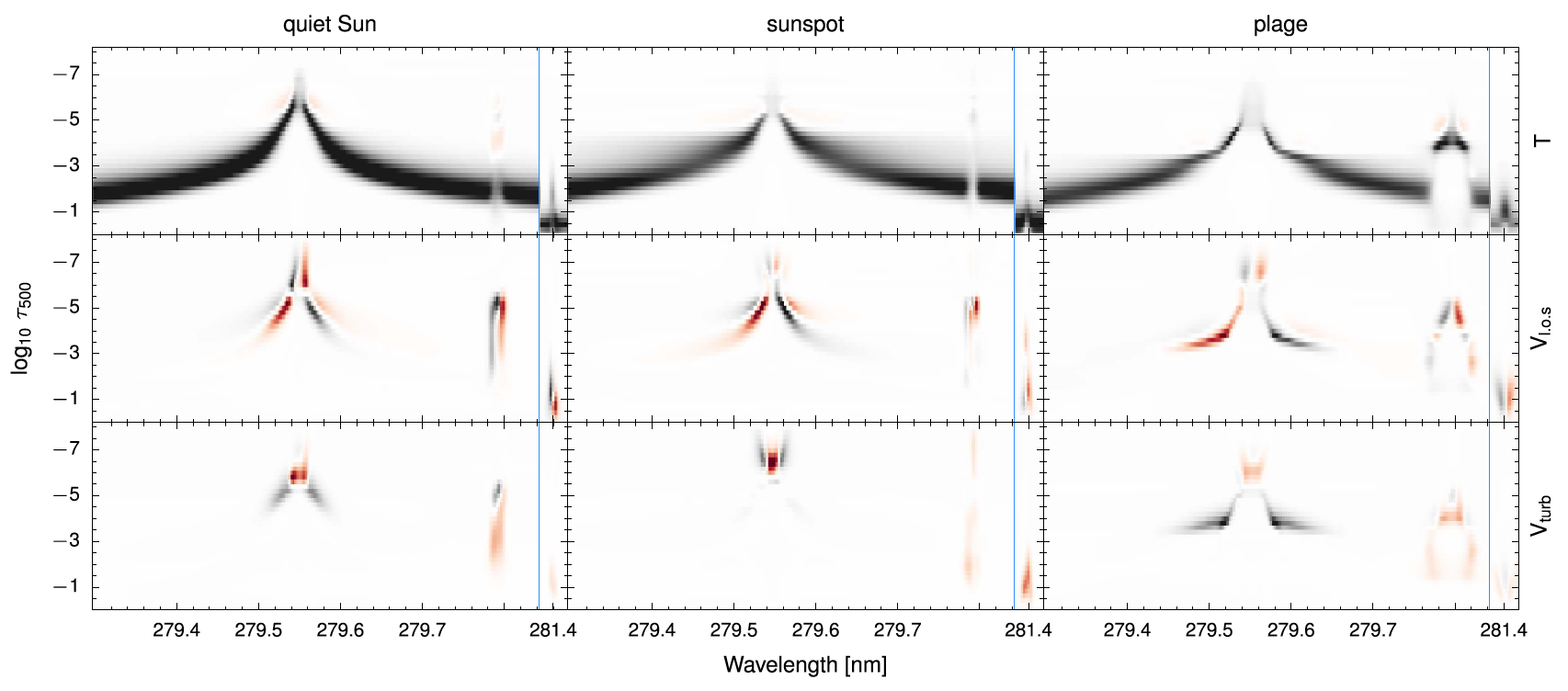
Figure 1.1 Response Functions of \(I\) to \(T, v_{los},\) and \(v_{turb}\) for the quiet-Sun, sunspot, and plage of inverted models with STiC in Mg II k lines (left-hand panel) and Mg II UV triplet (right-hand panel). Captured from de la Cruz Rodríguez et al 2019.
The uncertainties calculated by \(IRIS^{2}\) (see Eq. 2 in Sainz Dalda et al. 2019) are inversely proportional to the RFs. Nevertheless, it is important to understand the meaning of these uncertainties, i.e., to know where the observed lines are sensitive to a change in a physical variable. In those regions where the lines are most sensitive to a change in a physical variable the RF will be large, therefore the uncertainty will be small. One should keep that in mind when analyzing physical variables along the line of sight (optical depth) in the model atmosphere and their uncertainties.
While the Mg II h&k lines are optically thick on the disk, and probably off-limb to about 6 Mm as well, one must be careful when the observation is located near the limb. As the solar atmosphere is observed from disk center to limb, the optical ray goes along a more oblique trajectory, passing through a larger region of the atmosphere. In that case, the 3D effects have a greater impact on the formation (and the shape) of the line. As already mentioned, Sukhorukov & Leenaarts 2017 have shown that a proper modeling of Mg II h&k lines considering the center-to-limb variation requires the consideration of both 3D and PRD effects. This level of sophistication is currently not available in STiC inversions (which include multiatom, non-LTE, 1.5D and PRD effects), and therefore not in \(IRIS^{2}\) either. Thus, the inversion results provided by \(IRIS^{2}\) of observations close to the limb should be interpreted with caution.
1.3. Understanding the quality of the IRIS² results
It is important to understand how \(IRIS^{2}\) works in order to interpret the quality of the results provided. In that sense, knowing how \(IRIS^{2}\) looks for the closest RP in the \(IRIS^{2}\) datbase and how the noise of the original data is considered in the calculation of both \(\chi^2\) and the uncertainty of a physical paramater \(p\) (\(\sigma_p\)) is mandatory to understand the correct physical meaning of the results obtained.
1.3.1. The weights and the weighting windows: \(w_i\)
\(IRIS^{2}\) looks in the \(IRIS^{2}\) database for the profile that most closely matches the observed profile by considering a weighted Euclidean distance, as expressed by Equation 1:
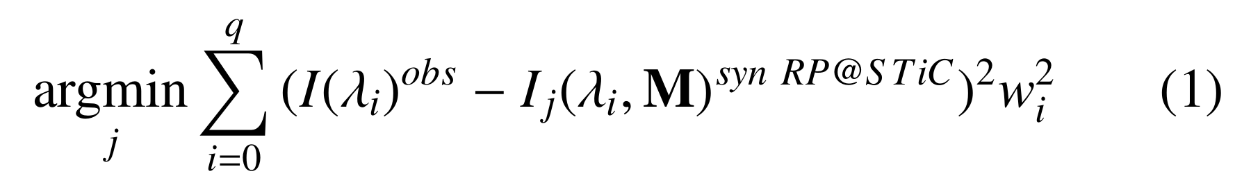
where \(j\) runs over all the synthetic RPs of the \(IRIS^{2}\) database, and \(w_{i}\) is a weight value given to either increase or decrease the contribution to the Euclidean distance of the intensity at the spectral position \(\lambda_{i}\). In pratice, the weights are given as a constant values to a set of spectral positions considered more important than others (e.g., to a spectral line of interest), or at spectral positions of less importance in (e.g., other lines not considered in our study). It is clear that weights have an effect on Eq. 1 only if they are different at different spectral positions: if \(w_i\) is the same for all \(\lambda_{i}\), then the Euclidean distance between the observed profile and the RP in the \(IRIS^{2}\) database is just scaled by factor of \(w_i = w\).

Figure 1.2 Top: An observed profile (in orange) and the same profile with constant weights \(w_i = [1., 1., 1., 1.]\) (solid blue) and when \(w_i = [1., 1/2., 1., 1/3.]\) (dashed blue). The weighting windows are displayed as: \(w_1\) (Mg k line, purple), \(w_2\) (Mg II UV, blue), \(w_3\) (Mg II h line, red), and \(w_4\) (some spectral positions in the bump between the Mg k and Mg h lines and the far red wing of Mg h line, yellow). Middle: Difference between the \(T, v_{los}, v_{turb},\) and \(n_{e}\) relative to the uncertainty when comparing the profile weighted with \(w_i = [1., 1., 1., 1.]\) with the original profile (blue lines), and comparing the profile weighted with \(w_i = [1., 1/2., 1., 1/3.]\) with the original profile (orange lines). Finally, the profile weighted with \(w_i = [1., 1., 1., 1.]\) is compared with respect to the profile weigthed with \(w_i = [1., 1/2., 1., 1/3.]\) (green lines). The lower panels show the same comparisons and their effect on the relative uncertainties of these physical variables. relative to the uncertainty of the reference profile (indicated by the supscript 0). The physical variables are the average values as a function of height in the full field of view of the active region used in Sainz Dalda et al. 2019. Click on the figure to enlarge it.
By default, \(IRIS^{2}\) considers all the spectral positions without any given weight, i.e. \(w_i = 1, \forall \lambda_i\). However, the user can change the weights in 4 pre-defined weighting
windows with the keyword weights_windows. The weighting windows are shown in the top panel of Fig. Figure 1.2. These windows weigh (if different values are given to the windows) the observed profile in the
following spectral ranges:
\(w_1\) (in purple): the Mg II k line, including its extended blue and red wings. An absorption line close to Mg II \(k_1v\) line is avoided.
\(w_2\) (in blue): the lines of the Mg II UV triplet located between the Mg II h&k lines.
\(w_3\) (in red): the Mg II h line, including its extended blue and red wings.
\(w_4\) (in yellow): the rest of the spectral positions corresponding to the bump between the Mg II h&k lines and some positions in the far red wing of Mg II h line.
The top panel of Figure 1.2 shows an original observed profile (orange), that observed profile weighted with \(w_i = [1., 1., 1., 1.]\) (blue), and the same observed profile weighted with \(w_i = [1., 1/2., 1., 1/3.]\) (dashed blue). Thus, in the last case, more attention is paid to the Mg II h&k lines with respect to the Mg II UV lines and the bump, i.e. we are overweighing the former with respect to the latter.
Warning
A value of weights_windows as [1,1/2,1/3,1] is interpreted by IDL as [1,0,0,1], while [1.,1/2.,1.,1/3.] is interpreted as
[1.00,0.50, 0.33, 1.00]. Therefore, if we want IDL to consider the weights as real numbers (float) it is mandatory to include the dot
(.) in the denominator of the weights (if they are given as a fractional number). In this manual we have intentionally kept
that notation as a reminder to the reader. For the sake of simplicity, weights_windows accepts an exception to a four element array as its input:
if weights_windows = 1, then iris2 code interprets that as weights_windows = [1., 1., 1., 1.].
1.3.2. The quality of the fit: \(\chi^2\)
To quantify the quality of the fit between the observed profile and the closest RP in the \(IRIS^{2}\) database we use \(\chi^2\), defined as:

where \(w_{i}\) and \(\sigma_{i}\) are the weight and the noise respectively at spectral position \(\lambda_{i}\), and \(\nu\) is the total number of spectral positions considered. The similarity between Eq. 1 and Eq. 2 is obvious: the main difference is that \(\chi^2\) considers the noise of the observed profile, and Eq. 1 does not.
\(\chi^2\) is a quantity integrated over all the spectral positions considered in the observed profile and the closest profile in the \(IRIS^{2}\) database. In most of the cases, this means that \(\chi^2\) evaluates the fit in more than one spectral line. Therefore, while we consider \(\chi^2\) as a valid quantity for evaluating the quality of the fit obtained by \(IRIS^{2}\), we strongly encourage the user to visually verify the fit between the observed profile and the profile in the \(IRIS^{2}\) database deemed closest by \(IRIS^{2}\) code.
As a rule of thumb, if the value of \(\chi^2\) is very large (i.e. \(\chi^2\) > 200) for a given fit, we
should consider the associated values of the atmosphere with great caution, perhaps even discarding
the results. If the value of \(\chi^2\) is intermediate (i.e. 50 < \(\chi^2\) < 200), a
visual comparison between the observed profile and the closest RP in the \(IRIS^{2}\)
database will help us to decide whether to retain or discard the corresponding results.
A small value of \(\chi^2\) (i.e. \(\chi^2\) < 50) usually guarantees a result that can be trusted. In any case,
inspecting the fit is always a good idea. The IDL function show_iris2model makes inspection an easy task
(see Section 2.5).
\(\chi^2\) is always provided by \(IRIS^{2}\) code, but the calibrated observed profiles and the closest
RPs found by \(IRIS^{2}\) are only given in the IDL output structure (iris2model) if the user
sets up the keyword level equals to 1 or 2 (see Section 2.4).
1.3.3. The uncertainty: \(\sigma_p\)
The uncertainty in a physical parameter \(p\) is given by:
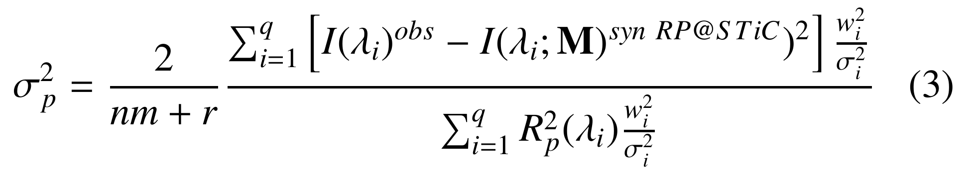
where \(R_p(\lambda_{i})\) is the response function of the Intensity at a given spectral position \(\lambda_{i}\) to a change in the physical parameter \(p\). In other words, the response function tells us how sensitive a given spectral position (or a set of positions, as in a spectral line) is to changes in the physical parameter.
The numerator of Eq. 3 is, except by the factor \(1/\nu\), equals to \(\chi^2\). Thefore, Eq. 3 can be interpreted as the ratio between the quality of the fit between the observed profile and the closest RP in the \(IRIS^{2}\) database, and how sensitive that closest RP is to changes in a physical parameter \(p\) of its associated RMA. Thus, the better the fit (i.e., the smaller the \(\chi^2\) value) the smaller the uncertainty; and the larger the senstivity of a line to changes in a physical parameter (i.e., large values of \(R_p(\lambda_i)\)) the smaller the uncertainty in this parameter.
Although \(\sigma_p\) could be calculated at each optical depth in the model, \(IRIS^{2}\) only calculates \(\sigma_p\) around those optical depths where the changes in the physical parameter of the model are allowed, i.e. in the vicinity of the nodes. While only calculated near the nodes, for consisitency with the model atmosphere provided by \(IRIS^{2}\), the uncertainty for each physical parameter is interpolated between the nodes to all the optical depths considered in the model.
The panels in the middle row of Figure 1.2 show the relative differences in the physical variables \(T, v_{los}, v_{turb}, n_e\) with respect to the uncertainty found in the reference profile (indicated by the supscript 0) where no weights applied and no windows subtracted from observed data (i.e. the orange profile in the upper panel). The results of this reference profile are compared to results obtained when the profiles are weighted with \(w_i = [1., 1., 1., 1.]\) (blue lines) and with \(w_i = [1., 1/2., 1., 1/3.]\) (orange lines). Also plotted are the relative differences in the same physical quanteties when considering the profiles weighted with \(w_i = [1., 1., 1., 1.]\) with respect to \(w_i = [1., 1/2., 1., 1/3.]\) respectively (green lines). The relative differences in the physical parameters when normalized to their uncertainties are very small (note the corresponding scales).
In the bottom panels, the relative difference between the uncertainties of these physical variables with respect to the uncertainty of the results obtained with the reference profiles are shown. We find that the relative differences may be as large as a -20% in the chromosphere (\(\log(\tau) < -4\)) when comparing the reference model uncertainties based on the the original profiles with both the weighted profiles. This means that in the chromosphere, the uncertainties of the results obtained with the weighted profiles are ~20% smaller (and therefore better) than the uncertaines using the original profiles. Comparing the uncertainties of the results obtained with the weighted profiles shows that the uncertainties are slightly smaller in \(v_{los}\) and in \(v_{turb}\) at all optical depths, and larger in the chromosphere in \(T\) and \(n_e\), for \(w_i = [1., 1., 1., 1.]\) than for the results obtained with \(w_i = [1., 1/2., 1., 1/3.]\) (green lines). However, note that for \(T\) and \(n_e\) the uncertainties in the chromosphere are much smaller for both the weighted profiles as compared to the original unweighted profile (blue and orange lines).
This example shows the effect that a set of weights may have in the physical parameters and their uncertainties. It is the user’s responsibility to choose a meaningful set of weights for his/her specific scientific goals.
1.4. IRIS² elements in SolarSoft
\(IRIS^{2}\) in IDL SolarSoft consists of three elements:
\(IRIS^{2}\) database: the version of the database is denoted in the file name with vN.M, with \(N, M \in \mathbb{N}\) (e.g., v2.0 contains version 2, revision 0). The files in the \(IRIS^{2}\) database are:
inv_mu_iris2.vN.M: this file includes the inverted RPs and the location on the solar disk where the RPs were observed, given as \(\mu=cos(\theta)\), being \(\theta\) the heliocentric angle. Thus, an element of this file is a vector with the intensity at 473 sampled wavelengths , i.e. the inverted RP, the \(\mu\) value is given in the 474th position of this vector. The meaning of their dimensions is: [\(\lambda_{IRIS{^2}}, RP_{IRIS^{2}}\ sample]\)
mod_iris2.vN.M: includes the corresponding Representative Model Atmospheres (RMA) resulting from the inversion of the observed RPs. Therefore, they are the RMAs that are able to reproduce (synthesize) the inverted RPs contained ininv_mu_iris2.vN.M. An element of this file is a 2D array containing the values of \(T[K],\ v_{los}[ms^{-1}], \ v_{turb}[ms^{-1}],\) and \(n_e[cm^{-3}]\) in a grid of 39 points in the optical depth range \(-7.6 < log(\tau) < 0.0\), i.e. each sample is an array of dimension 4x39. Thus, the meaning of their dimensions is: [\(p\), \(optical\ depth\ in\ log(\tau)\), \(RMA_{IRIS^{2}}\ sample\)], with \(p\) being the physical variables \(T[K],\ v_{los}[ms^{-1}], \ v_{turb}[ms^{-1}],\) and \(n_e[cm^{-3}]\).
nodes_var_nPP_iris2.vN.M(4 files): the location of the nodes with respect to the optical depths in the variablevarconsidered by STiC during the inversion of the RPs in the \(IRIS^{2}\) database. The textnPPindicates the number of nodes considered by STiC for that variable. For instance, nodes_temp_n07_iris2.v2.0.fits contains the positions of the nodes with respect to the optical depth (\(log(\tau)\)) considered for the inversion and the calculation of the response functions.vartext in the filename can be: ‘temp’, ‘vlos’, ‘vturb’, and ‘nne’.
rf_var_nPP_iris2.v.N.M(4 files): the response functions (RFs) obtained for each RP and RMA in the \(IRIS^{2}\) database. These response functions allow us to calculate the uncertainties (see Eq. 2 in Sainz Dalda et al. 2019). There are 4 of these files corresponding to the variables considered by \(IRIS^{2}\). The textnPPindicates the number of nodes used in the calculation of the RFs. Thus, ‘rf_temp_n07_iris2.v.2.0,fits’ means that the response function for the temperature has been computed in 7 nodes, the same number of nodes in \(T\) used by STiC in the last cycle of the inversion of the RPs. The meaning of their dimensions is: [\(\lambda_{IRIS{^2}}, nodes\ in\ the\ RMA_{IRIS^{2}}, RP_{IRIS^{2}}\ sample]\).
wl_iris2.v.N.M: the wavelengths of the inverted RPs in the \(IRIS^{2}\) database given ininv_mu_iris2.vN.M. Their units are \(Å\).
iris2 (IDL function): the function that actually makes the inversion, i.e. the match between an observed IRIS Mg II h&k profile and the closest inverted RP in the \(IRIS^{2}\) database. By default,iris2uses the full, latest version of the \(IRIS^{2}\) database, which is indicated by the name of the files, e.g. inv_mu_iris2.v2.0.fits. However, previous versions of the database can be used by setting the keywordversion_dbiniris2(see below). The user can constrain the RPs used from the \(IRIS^{2}\) database for the match between the observed profiles and the RPs to an interval in \(\mu\) centered around the \(\mu\) of the observation (see keyworddelta_mu). The minimal output of this function is a structure (or an array of structures) containing the model atmosphere and the uncertainties obtained from the inversion of the data passed byraster_files.
show_iris2model (IDL function): this function displays the output ofiris2. Points on the displayed image can be selected by the user (by pressingS). In which caseshow_iris2modelwill return the position of the selected points, their model atmospheres, their uncertainties, and other values.
Note
\(IRIS^{2}\) and \(deepIRIS^{2}\) are under development in python. All the information about how to use them in python will be available soon in |IRIS2| and |deepIRIS2| in python.
1.5. Acknowledging \(IRIS^{2}\)
If you use \(IRIS^{2}\) for your work in a publication, presentation, poster, or talk, we would appreciate it if you acknowledge it appropriately. For a publication, this is best done by citing the \(IRIS^{2}\) (Sainz Dalda et al. 2019) and STiC (de la Cruz Rodríguez et al 2019) papers.